
Cost Effectiveness of
Home Energy Retrofits in
Pre-Code Vintage Homes
in the United States
Philip Fairey and Danny Parker
BA-PIRC
November 2012

NOTICE
This report was prepared as an account of work sponsored by an agency of the
United States government. Neither the United States government nor any
agency thereof, nor any of their employees, subcontractors, or affiliated
partners makes any warranty, express or implied, or assumes any legal liability
or responsibility for the accuracy, completeness, or usefulness of any
information, apparatus, product, or process disclosed, or represents that its use
would not infringe privately owned rights. Reference herein to any specific
commercial product, process, or service by trade name, trademark,
manufacturer, or otherwise does not necessarily constitute or imply its
endorsement, recommendation, or favoring by the United States government
or any agency thereof. The views and opinions of authors expressed herein do
not necessarily state or reflect those of the United States government or any
agency thereof.
Available electronically at http://www.osti.gov/bridge
Available for a processing fee to U.S. Department of Energy
and its contractors, in paper, from:
U.S. Department of Energy
Office of Scientific and Technical Information
P.O. Box 62
Oak Ridge, TN 37831-0062
phone: 865.576.8401
fax: 865.576.5728
email: mailto:reports@adonis.osti.gov
Available for sale to the public, in paper, from:
U.S. Department of Commerce
National Technical Information Service
5285 Port Royal Road
Springfield, VA 22161
phone: 800.553.6847
fax: 703.605.6900
email: [email protected]world.gov
online ordering: http://www.ntis.gov/ordering.htm
Printed on paper containing at least 50% wastepaper, including 20% postconsumer waste

iii
Cost-Effectiveness of Home Energy Retrofits in
Pre-Code Vintage Homes in the United States
Prepared for:
The National Renewable Energy Laboratory
On behalf of the U.S. Department of Energy’s Building America Program
Office of Energy Efficiency and Renewable Energy
15013 Denver West Parkway
Golden, CO 80401
NREL Contract No. DE-AC36-08GO28308
Prepared by:
Philip Fairey and Danny Parker
BA-PIRC/Florida Solar Energy Center
1679 Clearlake Road, Cocoa, FL 32922
NREL Technical Monitor: Stacey Rothgeb
Prepared under Subcontract No. KNDJ-0-40339-02
October 2012
iv
[This page left blank]

v
Contents
List of Figures ............................................................................................................................................ vi
List of Tables .............................................................................................................................................. vi
Executive Summary ................................................................................................................................... ix
1 Introduction ........................................................................................................................................... 1
2 Methodology ......................................................................................................................................... 3
2.1 Archetypes ...........................................................................................................................3
3 Simulation Modeling ............................................................................................................................ 6
4 Other Considerations in the Optimizations ....................................................................................... 7
5 Economic Model ................................................................................................................................... 8
5.1 General Inflation Rate and Discount Rate ...........................................................................8
5.2 Optimization Method ...........................................................................................................9
5.3 Equipment Replacement ......................................................................................................9
6 Energy Price Rates ............................................................................................................................. 11
7 Retrofit Improvement Measures ........................................................................................................ 12
8 Improvement Cost Model ................................................................................................................... 16
9 Results ................................................................................................................................................. 24
9.1 Archetype Baseline Energy ................................................................................................24
10 Cost Optimization Results ................................................................................................................. 28
10.1 Optimization Scenario 1 ........................................................................................28
10.2 Optimization Scenario 2: Homeowner Financing ..................................................31
10.3 Optimization Scenario 3: HVAC Contractor Financing ........................................32
10.4 Optimization Scenario 4: Home Remodel Refinancing .........................................38
10.5 Method in Action: Optimization Results for a Specific Home ..............................40
11 Conclusions ........................................................................................................................................ 43
References ................................................................................................................................................. 46
Appendix A. Calculation of Economic Cost Effectiveness Section of RESNET Standards ........ 48
Appendix B. Determination of HVAC Equipment Costs .................................................................. 53
Appendix C. Optimization Scenario 1— Default Economic Parameter Model .............................. 57
Appendix D. Optimization Scenario 2— Homeowner Financing Home Improvement Loan Model69
Appendix E. Optimization Scenario 3— HVAC Contractor Financing Business Model .............. 79
Appendix F. Optimization Scenario 4— Home Remodel/Refinance .............................................. 89

vi
List of Figures
Figure 1. Histogram of achievable source energy reductions in 14 climates using four different
financing alternatives ........................................................................................................................... x
Figure 2. U.S. Census Bureau data on existing housing unit construction vintage by decade ........ 1
Figure 3. Median U.S. home size from U.S. Census Bureau data: 1973–2010 ...................................... 3
Figure 4. Starting screen for CostOpt ..................................................................................................... 22
Figure 5. Ft. Worth analysis using full costs for all measures and outright replacement ................ 34
Figure 6. Ft. Worth analysis using incremental costs (natural replacement costs) for all measures34
Figure 7. Source energy savings bins for the four optimization scenarios ........................................ 40
Figure 8. Optimization results for a specific home in Ft. Worth, Texas .............................................. 42
Figure 9. Results from regression analysis of CostOpt HVAC cost estimates .................................. 54
Figure 10. Comparison of CostOpt HVAC cost estimates and NREL HVAC cost estimates ............ 56
Unless otherwise noted, all figures were created by BA-PIRC.
List of Tables
Table 1. Pre-Code Vintage Existing Archetype Home Characteristics by IECC Climate Zone ........... 4
Table 2. Economic Parameter Values ....................................................................................................... 8
Table 3. Household Energy Cost Index .................................................................................................... 9
Table 4. Statewide Revenue-Based Energy Rates ................................................................................. 11
Table 5. Description of Retrofit Improvement Measures ...................................................................... 12
Table 6. Example Cost Calculations for 1600 ft
2
, Slab-on-Grade, Wood-Frame Archetype Home ... 18
Table 7. Calculation of Annual Maintenance Costs f8 or Specific Items ............................................ 21
Table 8. Comparison of Baseline Home Energy Uses With 2005 RECS Data ..................................... 24
Table 9. Archetype Descriptions, Locations, and Baseline Energy Uses and Costs ........................ 26
Table 10. Optimization Scenario 1—Default Economic Parameter Optimizations ............................. 29
Table 11. Optimization Scenario 2—Home Improvement Mortgage Optimizations ........................... 31
Table 12. Optimization Scenario 3—HVAC Replacement Optimizations ............................................ 37
Table 13. Optimization Scenario 4—Home Refinance Optimizations .................................................. 38
Table 14. Weighted Average Source Energy Savings and Average NPV for Four Optimization
Scenarios ............................................................................................................................................. 39
Table 15. NREL Cost Estimates for Heat Pumps ................................................................................... 55
Table 16. NREL Cost Estimates for Air Conditioners ............................................................................ 55
Table 17. NREL Cost Estimates for Gas Furnaces ................................................................................ 55
Unless otherwise noted, all tables were created by BA-PIRC.

vii
Definitions
ACH50
Air changes per hour
AEU
Average source energy use
AFUE
Annual fuel utilization efficiency
AHU
Air handling unit
ASHRAE
American Society of Heating, Refrigerating and Air Conditioning
Engineers
BEopt
Building Energy Optimization
CF
Cubic feet
cfm
Cubic feet per minute
CFL
Compact fluorescent lamp
CMU
Concrete masonry wall system
Crwl
Crawlspace foundation
CZ
Climate zone
DnPmt
Down payment rate
DR
Discount rate
EA
Number of each
EAC
Equivalent annual cost
EF
Energy factor
EIA
Energy Information Administration
ER
Energy inflation rate
FMC
Fixed measure cost
Frm
Frame wall system
GF
Gas furnace archetype (natural gas space and water heating)
GR
General inflation rate
GSF
Gross square feet
HEM
Home energy management
HP
Heat pump archetype (electric space and water heating)
HSPF
Heating seasonal performance factor
HVAC
Heating, ventilation, and air conditioning
HW
Hot water
IECC
International Energy Conservation Code

viii
kBtu
One thousand British thermal units
kWh
Kilowatts per hour
LED
Light-emitting diode
LF
Linear feet
MBtu
One million British thermal units
MMC
Minimum measure cost
MR
Mortgage interest rate
MURS
Minimum upgrade reference ratio
NPV
Net present value
NSF
Net square feet
pEA
Unit cost per each item (normally appliances, etc)
pCF
Unit cost per cubic foot (normally the house volume)
pGSF
Unit cost per gross square foot (normally for skin finish cost)
pLF
Unit cost per linear foot (normally the perimeter)
pNSF
Unit cost per net square foot (normally applied to walls only)
pSFpR
Unit cost per square foot per ΔR (normally blown insulation applied
to GSF)
PV
Photovoltaics
ΔR
R-value difference between existing home and improvement
measure
RECS
Residential Energy Consumption Survey
ReFi
Refinance
RESNET
Residential Energy Services Network
SEER
Seasonal energy efficiency ratio
SHGC
Solar heat gain coefficient
SIR
Savings-to-investment ratio
SOG
Slab-on-grade
StDev
Standard deviation
Sty
Story
TMC
Total measure cost
UC Bsmt
Unconditioned, unfinished basement foundation

ix
Executive Summary
This analytical study examined the opportunities for cost-effective energy efficiency and
renewable energy retrofits in residential archetypes constructed before 1980 (Pre-Code) in 14
U.S. cities. These cities represent each International Energy Conservation Code climate zone in
the contiguous United States.
The analysis was conducted using an in-house version of EnergyGauge USA v.2.8.05 named
CostOpt that was programmed to perform iterative, incremental economic optimization on a long
list of residential energy efficiency and renewable energy retrofit measures. The principal
objectives were to:
• Determine the opportunities for cost-effective source energy reductions in this large
cohort of existing residential building stock as a function of local climate and energy
costs.
• Examine how retrofit financing alternatives impact the source energy reductions that are
cost-effectively achievable.
A key finding was that the energy efficiency of even older, poorly insulated homes across U.S.
climates can be dramatically improved. Moreover, with favorable economics, they can reach
performance levels close to zero energy when evaluated on an annual source energy basis.
Findings indicated that retrofit financing alternatives and whether equipment requires
replacement had considerable impact on the achievable source energy reduction in this cohort of
residential building archetypes.
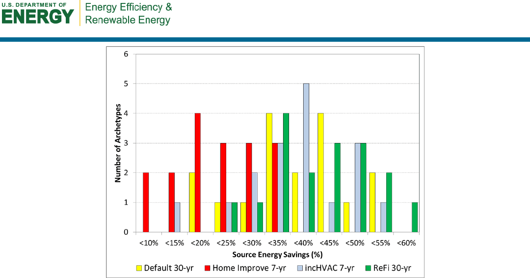
Figure 1 shows the study results. The four optimization scenarios examined are:
1. Default 30-yr. 30-year mortgage at 6.15% interest using full replacement cost
2. Home Improve 7-yr. 7-year mortgage at 6.15% interest using full replacement cost
3. incHVAC 7-yr. 7-year mortgage at 6.15% interest using incremental HVAC costs
4. ReFi 30-yr. 30-year refinance mortgage at 4.0% interest using full replacement costs.
x
Figure 1. Histogram of achievable source energy reductions in 14 climates
using four different financing alternatives
The figure shows that the standard short-term home improvement mortgage option seriously
restricts cost effectiveness. However, at the same time, if only the incremental costs of
replacement for heating, ventilation, and air-conditioning (HVAC) equipment are used in the
analysis (the HVAC equipment is no longer operational), a short term mortgage can result in
significant energy reductions. And, as expected, the home refinance option results in the largest
potential for source energy savings in this residential cohort.
If home energy retrofits and their attendant energy cost and environmental emission reductions
are considered advantageous to society as a whole, these results also have general policy
implications:
• HVAC contractors should be encouraged to take advantage of low incremental
replacement costs to substantially improve homes using short-term financing.
• Home refinance and resale opportunities offer a significant advantage to dramatically
improve home energy efficiency.
• The foreclosure marketplace and 30-yr mortgages should be a focus for home
improvement opportunities.
The findings relative to specific measures and how they perform across climates, utility costs,
and financing scenarios are:
• What works everywhere. Compact fluorescent lamps, duct sealing, ceiling insulation,
hot water tank wraps, low-flow fixtures.

xi
• What works in some places. Frame wall insulation, crawlspace wall insulation, solar
water heating, heat pump water heaters, photovoltaic systems, appliances that need
replacement and have low incremental costs.
• What does not work anywhere. Outright replacement of windows; most expensive
HVAC systems, and roof replacement.
1
1 Introduction
Many U.S. homes were constructed before the advent of building energy codes. In 1975, the
American Society of Heating, Refrigerating and Air-Conditioning Engineers (ASHRAE)
promulgated Standard 90-75, which is widely regarded as the first U.S. residential energy code.
Since that time, housing energy efficiency has significantly improved in many states. However,
pre-code housing remains a significant fraction of the nation’s housing stock.
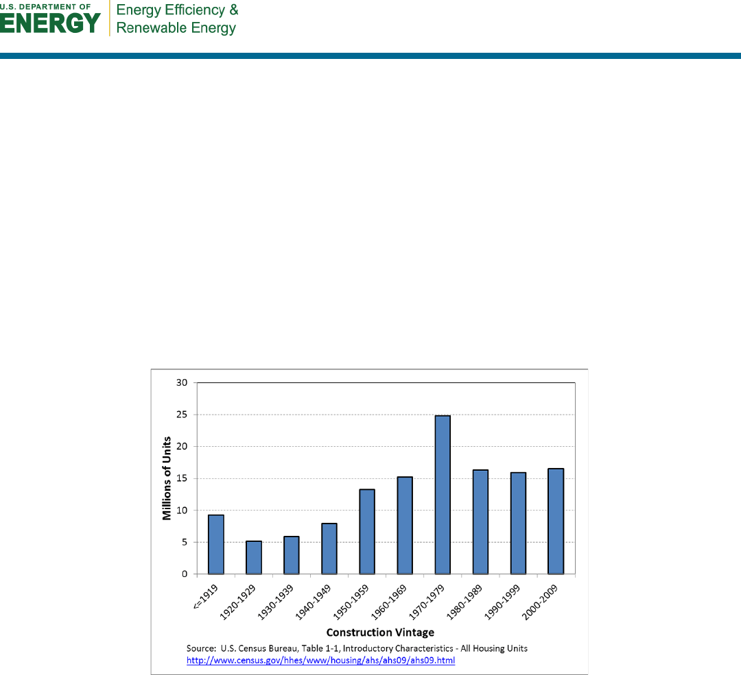
According to the U.S. Census Bureau, almost 25 million of the nation’s 130 million existing
housing units were built in the 1970s. The data comprising Figure 2 also show that more than
62% of existing housing was constructed before 1980, when building energy codes first began to
be adopted. A significant fraction of this stock includes components that have never been
improved since their original construction. Many comprise subdivisions and neighborhoods with
similar home designs and construction types. These neighborhoods provide significant
opportunities for targeted delivery of community-scale retrofit programs and projects.
Figure 2. U.S. Census Bureau data on existing
housing unit construction vintage by decade
This study investigates the cost effectiveness of a large number of potential home energy retrofit
measures using pre-code home archetypes that can be considered typical in a range of climates
throughout the United States. The analysis is conducted using an in-house optimization version
of EnergyGauge USA v.2.8.05 (EnergyGauge CostOpt) that has been configured to perform
economic cost-effectiveness analysis in accordance with recent standards (RESNET 2012).
Similar cost-effectiveness analysis was conducted by Casey and Booten (2011) using BEopt
software (Christensen et al. 2006; Polly et al. 2011). This investigation parallels this previous
work, using a somewhat different economic model specified by a recent RESNET Standard
(RESNET 2012). This study also uses home archetypes that vary from those used in the previous
analyses. For example, the previous study did not evaluate housing archetypes with concrete
masonry wall construction that is prevalent in the southeastern United States. This study also

2
allows fuel switching (changing from electric equipment to gas equipment and vice versa) and
examines how this can impact cost effectiveness under local climate and utility rate structures.
This investigation also directly analyzes solar hot water and solar photovoltaics (PV). Also,
contrary to the BEopt optimization scheme, the CostOpt method focuses on reductions to site
energy cost rather than source energy use, as this is what consumers pay.
3
2 Methodology
2.1 Archetypes
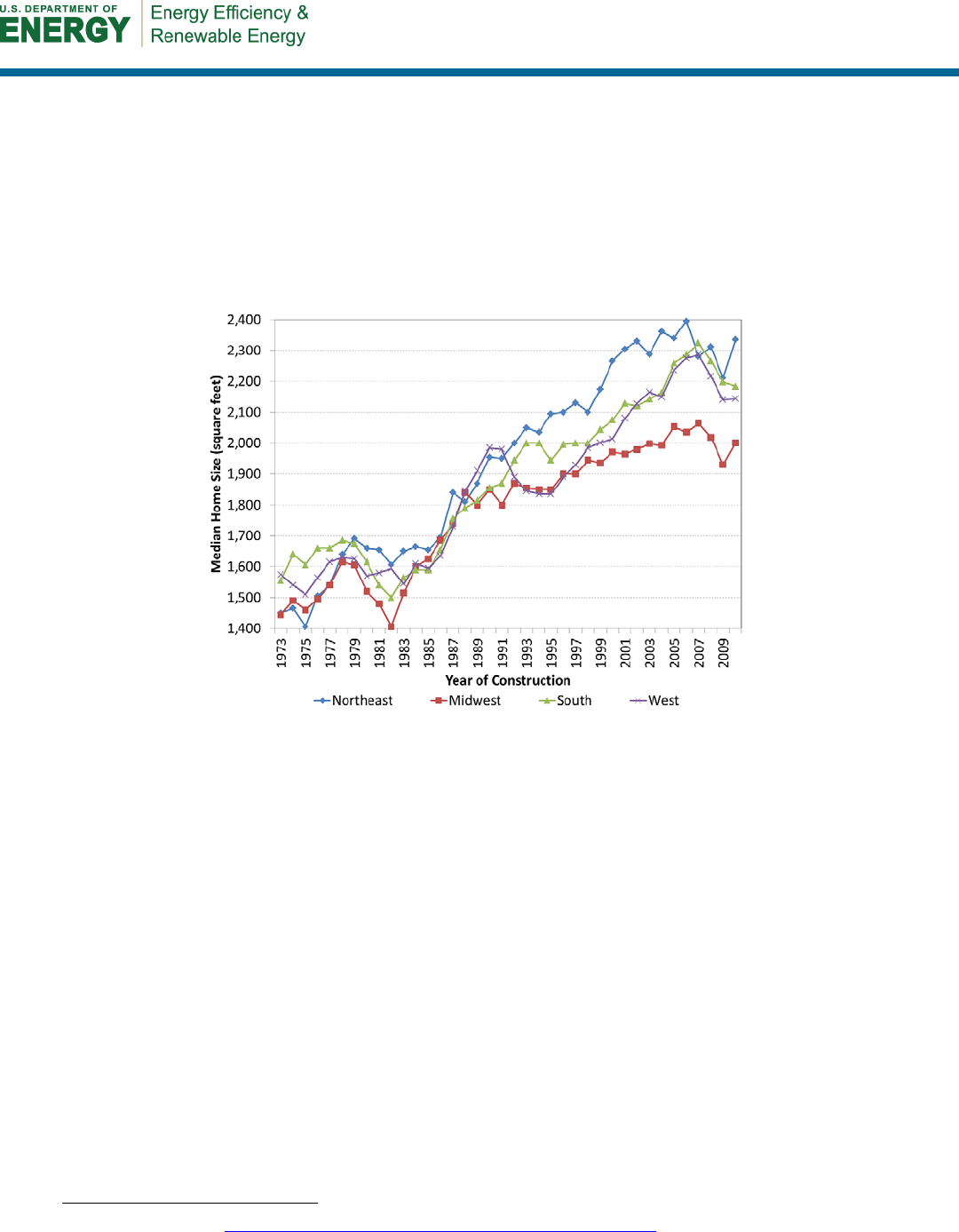
The archetype home characteristics used in this investigation are presented in Table 1. They are
largely characterized by the International Energy Conservation Code (IECC) climate zone in
which the archetype is located. At 1,600 ft
2
, the conditioned floor area is significantly smaller
than current practice but, according to the U.S. Census Bureau, this is consistent with homes
constructed before 1980 (see Figure 3).
1
Figure 3. Median U.S. home size from U.S. Census Bureau data: 1973–2010
These archetypes are similar to those used by Casey and Booten (2011) and by Parker et al.
(1998), but they differ in some important ways. In climate zone 1 (southern Florida), only
concrete masonry walls are considered and in climate zone 2 concrete masonry and frame wall
system are considered. Additionally, the assumed archetype envelope and duct air leakage
characteristics differ from those used by Casey and Booten. For example, Casey and Booten used
envelope air leakage of 19 ACH50 in all locations; this investigation uses 12, 9, and 7 ACH50 in
climate zones 1–2, 3–4, and 5–6, respectively. These much lower envelope leakage rates are
supported in part by data collected in Florida on a large number of existing homes (McIlvaine
2011) and are reasoned to more accurately characterize air leakage rates in other climates where
a significant cost penalty is incurred for very leaky homes, inducing homeowners to caulk and
weather strip their homes as matter of common do-it-yourself practice. That homes are somewhat
tighter in colder climates has also been observed in evaluations of large databases with tested fan
pressurization data (Sherman et al. 1986).
1
U.S. Census Bureau. http://www.census.gov/const/C25Ann/sftotalmedavgsqft.pdf

4
Table 1. Pre-Code Vintage Existing Archetype Home Characteristics by IECC Climate Zone
Archetype Characteristics
CZ 1-2
CZ 3-4
CZ 5-6
Conditioned floor area (ft
2
)
1,600
1,600
1,600
Foundation type
SOG
Crwl
UC Bsmt
AHU location
Garage
Crwl
UC Bsmt
Duct location
Attic
Crwl
UC Bsmt
Duct insulation R-value
4.2
4.2
4.2
Duct leakage (cfm25/ft
2
floor area)
0.11
0.11
0.08
Envelope ACH50
12
9
7
Roof solar absorptance
0.85
0.85
0.85
Wall solar absorptance
0.55
0.55
0.55
Ceiling R-value
10
15
20
Frame wall insulation R-value
1.5
5
7
Block wall insulation R-value
none
n/a
n/a
SOG perimeter R-value
none
n/a
n/a
Crawlspace floor R-value
n/a
5
n/a
Basement ceiling (house floor) R-value
n/a
n/a
none
Basement wall R-value
n/a
n/a
none
Window U-factor
1.2
0.75
0.6
Window SHGC
0.8
0.7
0.6
Door U-factor
0.5
0.4
0.3
HP HSPF (y2004; standard; degraded)
6.5
6.5
6.5
HP SEER (y2004; standard; degraded)
9.6
9.6
9.6
AC SEER (y2004; standard; degraded)
9.6
9.6
9.6
Furnace AFUE (y2004; standard; degraded)
76%
76%
76%
Gas HW EF (y2004; 40 gal; standard)
0.59
0.59
0.59
Elec HW EF (y2004; 40 gal; standard)
0.92
0.92
0.92
HW pipe insulation R-value
none
none
none
Lighting % fluorescent or equivalent
10%
10%
10%
Lighting kWh/yr
1,736
1,736
1,736
Refrigerator kWh/yr (y2004; 20 cf; SS/TDI)
717
717
717
Range/oven kWh/yr
447
447
447
Dishwasher kWh/yr (y2004; standard)
171
171
171
Clothes Washer kWh/yr (y2004; standard)
69
69
69
Clothes Dryer kWh/yr (y2004; standard)
970
970
970
Miscellaneous kWh/yr
2,000
2,000
2,000
Key to Table 1 abbreviations:
ACH 50: air changes per hour at a 50 Pascal pressure difference
AFUE: Annual fuel utilization efficiency
AHU: Air handling unit
CFM: Cubic feet per minute
Crwl: Crawlspace foundation
EF: Energy factor
HSPF: Heating seasonal performance factor
HW: Hot water
SEER: Seasonal energy efficiency ratio
SHGC: Solar heat gain coefficient
SS/TDI: Side-by-side, through the door ice
SOG: Slab-on-grade foundation
UC Bsmt: Unconditioned, unfinished basement foundation

5
Air distribution system leakage values are also supported by Walker (1998) and reinforced by
recent measured Florida data (McIlvaine 2011; Walker 1998). These rates are expected to be
consistent across a wide swath of the country. However, for the unconditioned basement
archetypes (climate zones 5 and 6) it is reduced to account for leakage in basements, which
results in significant regain and much less loss to the outdoors compared to cases where ducts are
located in vented attics or crawlspaces. For instance, recent work in Wisconsin in unconditioned
basement homes found that average tested duct leakage to the outside was only about 5% (Pigg
and Francisco 2006)—one third the typical leakage rate in homes with attic ducts.
Equipment efficiencies for the archetypes are based on the assumption that all equipment is 2004
vintage (currently 8 years old and halfway through its life expectancy) and is slightly degraded
using a maintenance factor of 0.005 (see Hendron 2006). Lighting and appliance energy uses are
based on the default values provided by RESNET (2012).

6
3 Simulation Modeling
The simulation analysis is conducted using EnergyGauge CostOpt, an implementation of
EnergyGauge USA v.2.8.05 with cost optimization capability. CostOpt uses an enhanced version
of DOE-2.1E to conduct detailed hourly simulations, including air distribution system leakage,
duct system heat transfer, improved HVAC systems modeling that includes improved relative
humidity (RH) and part load characterization as well as solar hot water and PV systems
performance prediction.
CostOpt performs cost optimization using an iterative incremental assessment method. The
analysis is “incremental” in that within any given category of improvement, such as insulation or
equipment efficiency, a number of options are presented to the software such that various
insulation values for each component, equipment efficiency, and their associated costs are
evaluated against each other simultaneously during each iteration. An iteration comprises a
simulation of each available improvement case on a measure-by-measure basis. At the
conclusion of each iteration, the improvement measure with the largest present value savings to
investment ratio (SIR; also known as the benefit to cost ratio) is incorporated into the home and
the remaining improvement measures are evaluated again on an incremental measure-by-
measure basis for the next iteration. This iterative process is continued until all available
measures that meet the user-specified SIR lower limit have been incorporated into the home.
CostOpt has been configured to “rank” measures within each iteration by net present value
(NPV). Although this option is not used in this investigation, it is often considered the economic
indicator of choice and, because it incorporates the improvement measures with the largest NPV
first, it passes over many measures that are incorporated incrementally and later improved by the
SIR ranking method. Thus, the NPV ranking method runs many fewer simulations (finishes
faster). Nonetheless, the SIR ranking method is chosen for this investigation for two reasons:
• It provides the incremental cost effectiveness of multiple options within a category of
measures (e.g., it will select R-19 ceiling insulation and then later replace it with R-30
insulation, usually installing other improvement measures).
• It provides an opportunity to answer an important question: What are the most cost-
effective improvement measures to select if one has only a limited budget? This is a
frequent constraint in many retrofit projects.

7
4 Other Considerations in the Optimizations
Other noteworthy simulation considerations:
• Optimization simulations generally allow fuel switching. The exception is in climate zone
1, where there is little, if any, reasonable access to residential natural gas.
• Gas furnaces (without an air conditioning component) were not allowed to compete in the
simulations if the baseline archetype did not contain a gas furnace. However, gas furnace-
air conditioner combinations were always allowed to compete in the simulations,
regardless of the equipment used for the baseline archetype.
• For the unconditioned basement homes, floor insulation (in the basement ceiling) was
limited to climate zone 5, where house floor insulation measures were allowed to
compete with basement wall insulation measures. For the coldest climate zone 6, floor
insulation was not allowed to compete out of concern that it could lower basement space
temperatures enough to allow freezing. In climate zone 6 archetypes, only basement wall
insulation was allowed as a basement thermal improvement.
• PV systems are evaluated assuming full net metering such that each kilowatt-hour the PV
system displaces is valued at the retail cost of electricity. This is true even when the PV
system produces more electricity than the home actually uses. This situation is seldom
encountered
• HVAC system sizing is dynamic in CostOpt. The building loads are calculated at the
beginning of each iteration using the building configuration resulting from previous
iterations. As a result, the building loads and required system capacity will decrease as
improvements are made. This, in turn, reduces HVAC improvement costs commensurate
with the reduction in building load and HVAC system capacity. HVAC measures are
much more likely to become cost effective following improvements than they are at the
start of the optimization.
8
5 Economic Model
CostOpt incorporates an economic model based on the Duffie and Beckman (1980) P1-P2
methodology. This procedure calculates two factors (P1 and P2) that can be applied
comprehensively to understand the cost effectiveness of energy-saving measures.
P1 is the ratio of the present value of the energy savings over the analysis period to the first year
energy cost savings. P2 is the ratio of the present value of the improvement costs over the
analysis period to the first cost of the improvement. In addition to standard rate parameters
(general inflation, fuel inflation, mortgage interest, and discount rate), both P1 and P2
incorporate the full range of applicable economic factors, including measure life, replacement
cost, maintenance cost, property tax cost, salvage value, and income tax benefit into their
calculation. As a result, if one knows the first cost of an energy improvement and the first year
energy saving of the improvement, the present value SIR of the improvement is simply P1 times
savings divided by P2 times cost. Likewise the NPV of the improvement is simply P1 times
savings minus P2 times cost. Furthermore, one can also calculate the break-even cost (the cost at
which SIR = 1) of an improvement given only the energy cost savings. This cost is simply P1
divided by P2 times the first year energy cost savings.
A large part of this model (except income tax benefit and property tax cost) has recently been
adopted by RESNET as part of its national consensus standard (RESNET 2012). In addition to
the economic model, the RESNET standard specifies a standard methodology of determining the
economic parameters values used in the model. The standard also dictates an economic analysis
period of 30 years. A full description of the RESNET implementation, which is used in this
investigation, is provided in Appendix A. In accordance with its standards, RESNET also
publishes the economic parameter values
2
that are intended for use in determining cost
effectiveness (see Table 2).
Table 2. Economic Parameter Values
General Inflation Rate (GR)
2.39%
Discount Rate (DR)
4.39%
Mortgage Interest Rate (MR)
6.15%
Down Payment Rate (DnPmt)
10.00%
Energy Inflation Rate (ER)
4.42%
The economic model used here differs from that proposed by Casey and Booten (2011) in
several important ways.
5.1 General Inflation Rate and Discount Rate
The model used in this investigation differentiates between the general inflation rate and the
discount rate; the model used by Casey and Booten sets them equal. The impact of setting these
two economic parameters equal is to say that the investor expects no return on investment.
However, it is not clear from Casey and Booten (2011) whether the discount rate they specify is
2
See http://www.resnet.us/standards/mortgage

9
the nominal discount rate or the real discount rate. For clarification, the discount rate provided in
Table 2 is taken as the nominal discount rate, making the real discount rate for the analysis
reported here equal to 1.95%.
The Casey and Booten analysis also appears to set the energy inflation rate equal to the general
inflation rate. The history of household energy costs during the past 10 years seems to contradict
this assumption. Table 3 presents U.S. Bureau of Labor Statistics data on the household energy
cost index since 2000.
3
These data show that household energy costs rose at an annual compound
rate of 4.42% between 2000 and 2010.
Table 3. Household Energy Cost Index
4
Year
2000
2001
2002
2003
2004
2005
2006
2007
2008
2009
2010
HHeI
122.8
135.4
127.2
138.2
144.4
161.6
171.1
181.7
200.8
188.1
189.3
HHeI = household energy cost index
Further evidence from the U.S. Energy Information Administration (EIA) shows that U.S.
average revenue-based residential electricity rate rose from $0.0824/kWh in 2000 to
$0.11.54/kWh in 2010. The annual compound rate for this rate change is 4.09%.
5.2 Optimization Method
The optimization method and philosophy used by BEopt (Polly et al. 2011) differ from that used
by CostOpt. BEopt ranks available improvement measures based on the least equivalent annual
cost (EAC) per percentage savings of annual average source energy use (AEU). Measures are
thus selected that emphasize source energy use savings. On the other hand, CostOpt uses
consumer-borne site energy costs, ranking available improvement measures based solely on the
life cycle present value SIR of the improvement measure over the analysis period. This results in
a different order of measure ranking and selection. Although source energy savings may be a
good societal objective, the methodology employed here reflects energy costs that will be best
appreciated by consumers.
5.3 Equipment Replacement
Another important methodological difference in the two methods is that BEopt assumes future
costs and energy savings for replacing equipment on burnout for the baseline home (Minimum
Upgrade Reference Scenario or MURS); CostOpt does not. Philosophically, the BEopt method
can be justified from the perspective that these costs and savings will occur at some time in the
future because equipment fails and minimum equipment standards may exceed those of the
equipment in the home. The BEopt cash flow analysis assumes that these future payments will be
in monies spent at the time of replacement and includes these payments (as well as the energy
savings they induce) in the equivalent annual energy cost calculation for the upgrade. As a result,
in the BEopt scenario, the equivalent annual cost for the MURS is higher than what consumers
would normally consider when they shop for the lowest cost improvement or the lowest
proposed bid.
3
These data used in determining economic parameter values in RESNET (2012).
4
U.S. Bureau of Labor Statistics, Table 3A. Consumer Price Index for all Urban Consumers (CPI-U): U.S. city
average, detailed expenditure categories http://www.bls.gov/cpi/cpi_dr.htm

10
The BEopt optimization analysis also allows this equipment to be replaced in the retrofit home in
year 1 using a finance mechanism (5 years at 7% in the case of the Casey and Booten analysis).
Thus, the cost of the year 1 replacement is effectively reduced by the difference between the
present value of the future equipment replacement cost in the MURS and the year 1 replacement
cost (including financing) in the retrofit case. Thus, older equipment will often be considered as
having a lower retrofit cost than the out-of-pocket expense for its replacement. The impact of this
assumption is large in the NREL assessment, as equipment and appliances are assumed to be
halfway through their useful service life.
This approach makes a credible academic argument (and a reasonable way to consider financing
from a societal perspective); however, in reality the full cost of any retrofit must be borne by the
homeowner at the time of replacement. Thus, discounting year 1 retrofit costs using the present
value of an anticipated future replacement cost does not bear on how much the home retrofit will
actually cost the consumer. On the contrary, consumers are often fixated on the out-of-pocket
costs of energy-related improvements, such that the CostOpt scheme better reflects homeowner
decision making.
CostOpt does not incorporate future upgrade costs and energy savings in the reference case.
Thus, the full improvement cost the consumer will face for the retrofit is used to calculate the
SIR for measure ranking and optimization. As a result, CostOpt is typically more conservative in
measure selection (especially for equipment upgrades) and is significantly more sensitive to the
financing term than BEopt, and longer term financing is significantly more productive than
short-term financing. We believe this better reflects the real constraints that most consumers
consider in choosing efficiency-related home improvement options.
11
6 Energy Price Rates
The CostOpt investigation uses statewide, revenue-based energy price rates derived from the
latest annual EIA databases
5,6
for residential electricity and natural gas, respectively. In some
instances (notably New York, California, and Maryland for electricity and New York, Arizona,
and Florida for natural gas) the EIA residential energy price rates differ substantially from those
used by Casey and Booten (2011). The energy price rates used for the 14 cities included in this
investigation are given in Table 4. These may differ from the specific utility costs in the various
locations, which could have a large impact on results. Further, the EIA utility revenue-based
rates do not include state, local, and municipality utility taxes, which are typically 5%–15%.
Thus, these rates are very conservative for our initial optimization assessment.
Table 4. Statewide Revenue-Based Energy Rates
City State CZ $/kWh $/therm
Miami
Florida 1 $0.1144 $1.844
Houston
Texas 2 $0.1160 $1.115
Atlanta
Georgia 3 $0.1007 $1.564
Los Angeles
California
3
$0.1475
$1.023
Seattle
Washington 4 $0.0804 $1.262
Phoenix
Arizona 2 $0.1097 $1.636
Minneapolis
Minnesota 6 $0.1059 $0.903
Detroit
Michigan 5 $0.1246 $1.167
New York
New York
4
$0.1874
$1.448
Ft. Worth
Texas 3 $0.1160 $1.115
San Francisco
California 3 $0.1475 $1.023
Denver
Colorado 5 $0.1104 $0.838
Baltimore
Maryland 4 $0.1432 $1.283
St. Louis
Missouri
4
$0.0908
$1.202
U.S. Average
$0.1154 $1.174
5
http://www.eia.gov/electricity/data.cfm#sales
6
http://www.eia.gov/dnav/ng/ng_pri_sum_dcu_STX_a.htm
12
7 Retrofit Improvement Measures
Ninety retrofit improvement measures are included in the analysis. Table 5 shows the acronyms
used for these measures and their descriptions. The category names in the second column are
used to affect the incremental analysis such that if two measures have the same category name,
they are effectively compared against one another on a cost differential basis. For example, if R-
19 ceiling insulation is accepted as the most cost-effective measure during the first iteration of
the optimization, the cost for all other ceiling insulation options during subsequent iterations is
equal to the difference in cost between the R-19 ceiling insulation that has already been accepted
and the cost of the other ceiling insulation options that remain on the list of potential
improvements. In this way, the various efficiency levels within a given category of measures are
incorporated only as they become cost effective, often with intervening measures from another
category incorporated in between.
Table 5. Description of Retrofit Improvement Measures
Acronym
Category
Description
SEER13HP
AC-HP
Minimum efficiency heat pump (SEER-13; HSPF-7.7)
SEER15HP
AC-HP
Improved efficiency heat pump (SEER-15; HSPF-9.0)
SEER18HP
AC-HP
High efficiency heat pump (SEER-18; HSPF-9.5)
SEER21HP
AC-HP
Very high efficiency heat pump (SEER-21; HSPF-10)
Mini-Split
AC-HP
Best efficiency mini-split heat pump (SEER-26; HSPF-
12)
SEER13AC
AC-SH
Minimum efficiency air conditioner with strip heat
(SEER-13; COP-1.0)
SEER15AC
AC-SH
Improved efficiency air conditioner w/ strip heat
(SEER-15; COP-1.0)
SEER18AC
AC-SH
High efficiency air conditioner with strip heat
(SEER-18; COP-1.0)
SEER21AC
AC-SH
Very high efficiency air conditioner with strip heat
(SEER-21; COP-1.0)
SEER13GF80
AC-GF
Minimum efficiency gas furnace/minimum efficiency air
conditioner (SEER-13; AFUE-80)
SEER13GF90
AC-GF
Improved efficiency gas furnace/minimum efficiency air
conditioner (SEER-13; AFUE-90)
SEER13GF96
AC-GF
High-efficiency gas furnace/minimum efficiency air
conditioner (SEER-13; AFUE-96)
SEER15GF90
AC-GF
Improved efficiency gas furnace/improved efficiency air
conditioner (SEER-15; AFUE-90)
SEER15GF96
AC-GF
High efficiency gas furnace/improved efficiency air
conditioner (SEER-15; AFUE-96)
SEER18GF96
AC-GF
High efficiency gas furnace/high efficiency air conditioner
(SEER-18; AFUE-96)
AFUE-80
GF
Minimum efficiency gas furnace (AFUE-80)
AFUE-90
GF
Improved efficiency gas furnace (AFUE-90)
AFUE-96
GF
High efficiency gas furnace (AFUE-96)
SealDucts
Ducts
Seal ducts to 6 cfm25-out per 100 ft
2
conditioned floor
13
Acronym
Category
Description
area
LeakFree
Ducts
Substantially leak free ducts at 3 cfm25-out per 100 ft
2
conditioned floor area
IntDucts
Ducts
Install substantially leak-fee ducts inside the conditioned
space
IntAHU
Move air handler unit to inside the conditioned space
Ceil_R11
Ceiling_Ins
Insulate ceiling to R-11
Ceil_R16
Ceiling_Ins
Insulate ceiling to R-16
Ceil_R19
Ceiling_Ins
Insulate ceiling to R-19
Ceil_R30
Ceiling_Ins
Insulate ceiling to R-30
Ceil_R38
Ceiling_Ins
Insulate ceiling to R-38
Ceil_R49
Ceiling_Ins
Insulate ceiling to R-49
Ceil_R60
Ceiling_Ins
Insulate ceiling to R-60
WhShngl
Roof
Replace roof shingles with white shingles (solar
absorptance = 0.75)
DrkShngl
Roof
Replace roof shingles with dark shingles
(solar absorptance = 0.92)
Wht Roof
Roof
Install a white metal roof (solar absorptance = 0.30)
RBS
Install an attic radiant barrier system
CrwlFl_R11
CrwlFloor_ins
Insulate floor between crawlspace and conditioned space
to R-11
CrwlFl_R19
CrwlFloor_ins
Insulate floor between crawlspace and conditioned space
to R-19
CrwlFl_R30
CrwlFloor_ins
Insulate floor between crawlspace and conditioned space
to R-30
SOG_R5-2h
SOG_ins
Insulate slab perimeter edge to R-5; 2 ft deep
SOG_R5-4h
SOG_ins
Insulate slab perimeter edge to R-5; 4 ft deep
Tile Floor
SOG_Floors
Install tile floors on slab
Carpet
SOG_Floors
Install carpet floors on slab
Wood Floor
SOG_Floors
Install wood floors on slab
BsmtFl_R11
BsmtFloor_ins
Insulate floor between unconditioned basement and
conditioned space to R-11
BsmtFl_R19
BsmtFloor_ins
Insulate floor between unconditioned basement and
conditioned space to R-19
BsmtFl_R30
BsmtFloor_ins
Insulate floor between unconditioned basement and
conditioned space to R-30
CMU_R5
CMU_Ins
Add R-5 exterior insulation to concrete masonry walls
CMU_R10
CMU_Ins
Add R-10 exterior insulation to concrete masonry walls
FrmW_R13
FrameWall_ins
Insulate exterior frame walls to R-13 (drill and fill)
FrmW_R18
FrameWall_ins
Insulate exterior frame walls to R-18 (drill and fill +
insulation sheathing + skin)
CrwlW_R5
CrwlWall_ins
Insulate crawlspace walls to R-5 (includes sealing
crawlspace)
CrwlW_R10
CrwlWall_ins
Insulate crawlspace walls to R-10 (includes sealing
crawlspace)
14
Acronym
Category
Description
CrwlW_R15
CrwlWall_ins
Insulate crawlspace walls to R-15 (includes sealing
crawlspace)
Crwl_noVnt
CrwlWall_ins
Seal vented crawlspace (includes required ground cover)
BsmtW_R11
BsmtWall_ins
Insulate unconditioned basement walls to R-11
BsmtW_R19
BsmtWall_ins
Insulate unconditioned basement walls to R-19
BsmtW_R30
BsmtWall_ins
Insulate unconditioned basement walls to R-30
Lgtwalls
Paint exterior walls light color (solar absorptance = 0.40)
Darkwalls
Paint exterior walls dark color (solar absorptance = 0.70)
Tight
Infiltration
Air seal to ACH50 = 7
Tighter
Infiltration
Air seal to ACH50 = 5
VTight
Infiltration
Air seal to ACH50 = 3
StrmWin
Windows
Add storm windows
WinTint
Windows
Add window tint film to windows
SGreflect
Windows
Replace with single-pane reflective windows
(U = 0.78; SHGC = 0.24)
DGLES
Windows
Replace with double-pane low-e solar windows
(U = 0.39; SHGC = 0.28)
DGLEH
Windows
Replace with double-pane low-e heating windows
(U = 0.39; SHGC = 0.52)
DGLEArH
Windows
Replace with double-pane low-e, argon heating windows
(U = 0.29; SHGC = 0.48)
DGLEArS
Windows
Replace with double-pane low-e, argon solar windows (U
= 0.29; SHGC = 0.24)
TGLEArH
Windows
Replace with triple-pane low-e, argon heating windows (U
= 0.20; SHGC = 0.43)
Lgts_50%
Lighting
Install 50% high efficiency lighting
Lgts_75%
Lighting
Install 75% high efficiency lighting
Lgts_100%
Lighting
Install 100% high efficiency lighting
HWwrap
Add R-10 hot water tank wrap
LowFloSh
Replace shower heads with low-flow shower heads
Std_EHW
Water_Heater
Replace with minimum standard electric hot water system
(EF = 0.92)
Std_GHW
Water_Heater
Replace with minimum standard gas hot water system (EF
= 0.59)
ES_GHW
Water_Heater
Replace with ENERGY STAR gas hot water system (EF
= 0.62)
TGWH
Water_Heater
Replace with tankless gas hot water system (EF = 0.82)
SHW_40/80PV
SolarHW
Replace with 40-ft
2,
80-gal, PV-pumped solar hot water
system
SHW_ICS40
SolarHW
Replace with 40-gal, integrated collector storage solar hot
water system
SHW_ICS-HP
SolarHW
Replace with 40-gal ICS solar hot water system with
HPWH backup
HRUnit
Install hot water heat recovery unit on HVAC system
HPWH
HPWH
Install heat pump hot water heater (COP = 2.0)
15
Acronym
Category
Description
Dryer
Dryer
Replace with high efficiency clothes dryer
(809 kWh/yr)
ES_Fridge
Replace with ENERGY STAR refrigerator
(460 kWh/yr)
ES_dWash
Replace with ENERGY STAR dishwasher (EF = 0.68)
ES_Washer
Replace with ENERGY STAR washer
(washer = 123 kWh/yr; dryer = 618 kWh/yr)
Misc/HEM
Misc
Home energy management (reduces lighting and
appliance use by 480 kWh/yr)
WHFan
Install whole-house ventilation fan (produces 2.5 ACH
ventilation when running)
PipeIns
Add R-2 Insulation to exposed hot water piping
Ins_Door
Replace exterior doors with insulated doors (U = 0.29)
5kW-PV
PV
Install 5-kW PV system

16
8 Improvement Cost Model
In most cases, improvement costs used in this investigation parallel those available from the
National Renewable Energy Laboratory’s (NREL) National Residential Efficiency Measure
Database.
7
However, this study includes measures for which costs are not available in the NREL
database (such as solar water heating and PV).
For heating and air conditioning equipment, costs were incorporated based on a separate study
whereby the costs are expressed in an equation as a function of the equipment capacity and
efficiency along with an offset. The data and analysis that underlie these heating and cooling
equipment cost equations are presented in Appendix B. For certain other costs, the NREL cost
data were reduced to equations based on component areas and incremental improvement
changes. For example, examination of the NREL data on fibrous insulation reveals that the cost
of fibrous insulation is approximately $0.035/ft
2
per R-value. For these types of improvements
these costs were cast in such terms. For most other costs, the costs contained in the NREL
database were adopted.
For HVAC equipment, CostOpt uses the following equations to calculate installed retrofit costs
(see also Appendix B for derivations).
• Heat pumps: –5539 + 604*SEER + 699*tons
• Air conditioners (with strip heat): –1409 + 292*SEER + 520*tons
• Gas furnace/air conditioner: –6067 + 568*SEER + 517*tons + 4.04*kBtu + 1468*AFUE
• Gas furnace only: –3936 + 14.95*kBtu + 5865*AFUE
where:
tons = air conditioning capacity
kBtu = gas furnace capacity, which is limited to a minimum value of 45
The estimating equations are valid for heat pump and cooling system sizes of 1.5–5 tons and
multiples thereof. Similarly, the costs of gas heating equipment are based on capacities of 40–
120 kBtu/h.
For other options, costs depend on either the building configuration or the quantity of items
required. We generally use the following equation to define measure costs as a function of the
home geometry or number of items required.
TMC = FMC + (pSFpR*ΔR*GSF) + (pNSF*NSF) + (pGSF*GSF) + (pLF*LF) + (pCF*CF) + (pEA*EA)
or MMC, whichever is less
where:
TMC =
Total measure cost ($)
FMC = Fixed measure cost (coming out charge, etc.)
MMC = Minimum measure cost (cost below which the measure will not be implemented)
pSFpR = Unit cost per square foot per ΔR (normally blown insulation applied to GSF)
7
www.nrel.gov/ap/retrofits/index.cfm

17
ΔR = R-value difference between existing home and improvement measure
GSF = Gross square feet
pNSF = Unit cost per net square foot (normally applied to walls only)
NSF = Net square feet
pGSF = Unit cost per gross square foot (normally for skin finish cost)
pLF = Unit cost per linear foot (normally the perimeter)
LF = Linear feet
pCF = Unit cost per cubic foot (normally the house volume)
CF = Cubic feet
pEA = Unit cost per each item (normally appliances, etc.)
EA = Number of each
Table 6 presents an example of the measure cost determination used by CostOpt. Where the
measure cost is shown as $0, there is no construction component for the specific home being
modeled.
18
Table 6. Example Cost Calculations for 1600 ft
2
, SOG, Wood-Frame Archetype Home
RunName
MeasureCost
MeasureLife
Incentive
IncrementalCost
MaintFrac
IncBasis
(fullCost - IncBasis
= incCost)
MMC (min measure cost)
FMC (fixed measure cost)
pSFpR (per sq.ft. per ΔR)
units of pSFpR
ΔR-value
pNSF (per net sq.ft.)
units of pNSF
pGSF (per gross sq.ft.)
units of pGSF
pLF (per linear ft.)
units of pLF
pCF
(per cu.ft.)
units of PCF
pEA
(per each item)
units of EA
description of EA
SealDucts
$500
20
$0
$500
0
$1.25
400
LeakFree
$900
20
$0
$900
0
$2.25
400
IntDucts
$6,400
50
$0
$6,400
0
$4.00
1600
IntAHU
$1,600
15
$0
$1,600
0
$1.00
1600
Ceil_R11
$300
50
$0
$300
0
$300
$0.035
1600
1
Ceil_R16
$336
50
$0
$336
0
$300
$0.035
1600
6
Ceil_R19
$504
50
$0
$504
0
$300
$0.035
1600
9
Ceil_R30
$1,120
50
$0
$1,120
0
$300
$0.035
1600
20
Ceil_R38
$1,568
50
$0
$1,568
0
$300
$0.035
1600
28
Ceil_R49
$2,184
50
$0
$2,184
0
$300
$0.035
1600
39
Ceil_R60
$2,800
50
$0
$2,800
0
$300
$0.035
1600
50
KneeW_R11
$0
50
$0
$0
0
$300
$0.035
0
11
$0.75
0
KneeW_R19
$0
50
$0
$0
0
$300
$0.035
0
19
$0.75
0
KneeW_R30
$0
50
$0
$0
0
$300
$0.035
0
30
$0.75
0
KneeW_R38
$0
50
$0
$0
0
$300
$0.035
0
38
$0.75
0
CathC_R11
$0
50
$0
$0
0
$300
$0.035
0
11
$2.00
0
CathC_R19
$0
50
$0
$0
0
$300
$0.035
0
19
$2.00
0
CathC_R30
$0
50
$0
$0
0
$300
$0.035
0
30
$2.00
0
CathC_R38
$0
50
$0
$0
0
$300
$0.035
0
38
$2.00
0
CathC_R49
$0
50
$0
$0
0
$300
$0.035
0
49
$2.00
0
WhShngl
$3,200
15
$0
$10
3,190
$2.00
1600
DrkShngl
$3,200
15
$0
$10
3,190
$2.00
1600
Wht Roof
$11,200
30
$0
$8,000
3,200
$7.00
1600
RBS
$2,400
30
$0
$800
1,600
$1.50
1600
CrwlFl_R11
$0
50
$0
$0
0
$0.035
0
11
$0.75
0
CrwlFl_R19
$0
50
$0
$0
0
$0.035
0
19
$0.75
0
CrwlFl_R30
$0
50
$0
$0
0
$0.035
0
30
$0.75
0
RasdFl_R11
$0
50
$0
$0
0
$0.035
0
11
$2.50
0
RasdFl_R19
$0
50
$0
$0
0
$0.035
0
19
$2.50
0
RasdFl_R30
$0
50
$0
$0
0
$0.035
0
30
$2.50
0
FOGar_R11
$0
50
$0
$0
0
$0.035
0
11
$2.50
0
FOGar_R19
$0
50
$0
$0
0
$0.035
0
19
$2.50
0
FOGar_R30
$0
50
$0
$0
0
$0.035
0
30
$2.50
0
SOG_R5-2h
$820
50
$0
$820
0
$5.00
164
SOG_R5-4h
$1,148
50
$0
$1,148
0
$7.00
164
Tile Floor
$4,480
50
$0
$4,480
0
$4.00
1120
Carpet
$3,520
50
$0
$3,520
0
$2.75
1280

19
RunName
MeasureCost
MeasureLife
Incentive
IncrementalCost
MaintFrac
IncBasis
(fullCost - IncBasis
= incCost)
MMC (min measure cost)
FMC (fixed measure cost)
pSFpR (per sq.ft. per ΔR)
units of pSFpR
ΔR-value
pNSF (per net sq.ft.)
units of pNSF
pGSF (per gross sq.ft.)
units of pGSF
pLF (per linear ft.)
units of pLF
pCF
(per cu.ft.)
units of PCF
pEA
(per each item)
units of EA
description of EA
Wood Floor
$5,320
50
$0
$5,320
0
$4.75
1120
BsmtFl_R11
$0
50
$0
$0
0
$300
$0.055
0
11
BsmtFl_R19
$0
50
$0
$0
0
$300
$0.055
0
19
BsmtFl_R30
$0
50
$0
$0
0
$300
$0.055
0
30
CMU_R5
$0
50
$0
$0
0
0.96
0
$5.50
0
CMU_R10
$0
50
$0
$0
0
1.10
0
$5.50
0
FrmW_R13
$3,225
50
$0
$3,225
0
$0.035
1032
13
$2.10
1312
FrmW_R18
$6,177
50
$0
$6,177
0
$0.035
1032
13
$4.35
1312
CrwlW_R5
$0
50
$0
$0
0
1.71
0
$1.00
0
CrwlW_R10
$0
50
$0
$0
0
1.85
0
$1.00
0
CrwlW_R15
$0
50
$0
$0
0
2.25
0
$1.00
0
Crwl_noVnt
$0
50
$0
$0
0
$1.00
0
BsmtW_R11
$0
50
$0
$0
0
$0.035
0
11
$2.00
0
BsmtW_R19
$0
50
$0
$0
0
$0.035
0
19
$2.00
0
BsmtW_R30
$0
50
$0
$0
0
$0.035
0
30
$2.00
0
Lgtwalls
$656
15
$0
$10
646
$0.50
1312
Darkwalls
$656
15
$0
$10
646
$0.50
1312
Tight
$320
20
$0
$320
0
$300
$0.025
12,800
Tighter
$1,280
20
$0
$1,280
0
$0.100
12,800
VTight
$2,560
20
$0
$2,560
0
$0.200
12,800
StrmWin
$2,400
20
$0
$2,400
0
$10.00
240
WinTint
$1,500
10
$0
$1,500
0
$6.25
240
SGreflect
$6,720
50
$0
$240
6,480
$28.00
240
DGLES
$7,200
50
$0
$720
6,480
$30.00
240
DGLEH
$7,200
50
$0
$720
6,480
$30.00
240
DGLEArH
$8,160
50
$0
$1,680
6,480
$34.00
240
DGLEArS
$8,160
50
$0
$1,680
6,480
$34.00
240
TGLEArH
$14,400
50
$0
$7,920
6,480
$60.00
240
Lgts_50%
$120
5
$0
$120
0
$0.08
1600
Lgts_75%
$240
5
$0
$240
0
$0.15
1600
Lgts_100%
$400
5
$0
$400
0
$0.25
1600
HWwrap
$50
12
$0
$50
0
$50
1
HWtank
LowFloSh
$70
15
$0
$70
0
$35
2
shower
Std_EHW
$408
12
$0
$10
398
$408
1
system
Std_GHW
$700
12
$0
$292
408
$700
1
system
ES_GHW
$750
12
$0
$342
408
$750
1
system
TGWH
$950
12
$0
$542
2.41%
408
$950
1
system
SHW_40/80
PV
$6,000
40
$1,800
$5,592
1.13%
408
$6,000
1
system
SHW_ICS40
$4,500
40
$1,350
$4,092
0.42%
408
$4,500
1
system
20
RunName
MeasureCost
MeasureLife
Incentive
IncrementalCost
MaintFrac
IncBasis
(fullCost - IncBasis
= incCost)
MMC (min measure cost)
FMC (fixed measure cost)
pSFpR (per sq.ft. per ΔR)
units of pSFpR
ΔR-value
pNSF (per net sq.ft.)
units of pNSF
pGSF (per gross sq.ft.)
units of pGSF
pLF (per linear ft.)
units of pLF
pCF
(per cu.ft.)
units of PCF
pEA
(per each item)
units of EA
description of EA
SHW_ICS-
HP
$6,000
40
$1,800
$5,592
1.44%
408
$6,000
1
system
HRUnit
$1,500
15
$0
$1,500
0
$1,500
1
HRU
HPWH
$1,900
15
$300
$1,492
1.05%
408
$1,900
1
HPWH
Pstat
$150
15
$0
$150
0
$150
1
stat
cFan
$1,080
20
$0
$400
680
$270
4
Nbr+1
Dryer
$800
15
$0
$100
700
$800
1
dryer
ES_Fridge
$1,000
15
$0
$100
900
$1,000
1
fridge
ES_dWash
$400
15
$0
$75
325
$400
1
dWash
ES_Washer
$1,200
15
$0
$200
1,000
$1,200
1
cWash
Misc/HEM
$600
10
$0
$600
0
$600
1
system
WHFan
$2,350
10
$0
$2,350
0
$1,175
2
fan
PoolPump
$0
15
$0
$0
0
$320
0
pump
WellPump
$0
15
$0
$0
0
$150
0
pump
Cln_FrigCoil
$30
3
$0
$30
0
$30
1
fridge
PipeIns
$40
15
$0
$40
0
$40
1
pipe ins
Ins_Door
$600
40
$0
$250
350
$300
2
door
5kW-PV
$32,500
40
$9,750
$32,500
1.58%
0
$6.50
5,000
wattsPV
21
The maintenance fractions given as a percent in Table 6 are equal to the annual maintenance cost
divided by the measure cost. Maintenance fractions are useful for describing differential
maintenance costs as compared with the standard practice and are also a good way to include
added costs for items in a system that do not last the full life of the longest lasting components of
the system, such as solar systems where pumps and tanks need replacement much more often
than the collector. They also allow for incorporation of performance degradation factors such as
those that occur in PV systems. The maintenance fractions used by CostOpt in this investigation
are shown in Table 7.
Table 7. Calculation of Annual Maintenance Costs for Specific Items
RunName
maint$/year
maint$_#1
maintPeriod_#1
maint$_#2
maintPeriod_#2
maint$_#3
maintPeriod_#3
Comments/Notes
TGWH
$22.92
$25
1
$25/yr for cleaning
SHW_40/80PV
$67.50 $150 5 $300 10 $750 20
$150 every 5 yrs for
pump + $300 every 10 yrs
for tank + $750 every 20
yrs for reroofing
SHW_ICS40
$18.75 $750 20
$750 every 20 yrs to
remove and replace for
reroofing
SHW_ICS-HP
$86.67 $750 20 $1,000 15 $150 5
$750 every 20 yrs to
remove and replace for
reroofing + replace
HPWH every 15 yrs +
150 every 5 yrs for
HPWH
HPWH
$20
$150
5
$150 every 5 yrs
5kW-PV
$350 $4,000 10 $2,000 20
$0.80/W for new inverter
every 10 yrs + $0.40/W
every 20 yrs for reroofing
+ 0.5% PV degradation
22
CostOpt also provides two operational “flags” for each measure that control the simulations. One
is a simulation flag controlling whether a given measure is included in the list of measures to be
simulated. If the measure cost evaluates to $0 (see Table 6 for examples), this flag is
automatically set to false and the measure is not included in the list of measures evaluated.
However, users can manipulate the simulation flag to reduce the number of simulations
performed when they know that a measure is highly unlikely to be cost effective or if they do not
want to consider the measure for aesthetic or practical reasons.
The second flag is the incremental cost flag, which indicates that incremental cost should be used
to evaluate the measure because the option is at the end of its service life and must be replaced.
This flag defaults to false for all measures. However, users can set this flag to true on a measure
by measure basis, allowing measures to be evaluated on an incremental cost basis rather than a
full cost basis. For example, if the HVAC equipment is no longer operational and will be
replaced, the incremental flag for HVAC equipment can be set to true and the incremental cost
rather than the full cost will be used by CostOpt in the optimization.
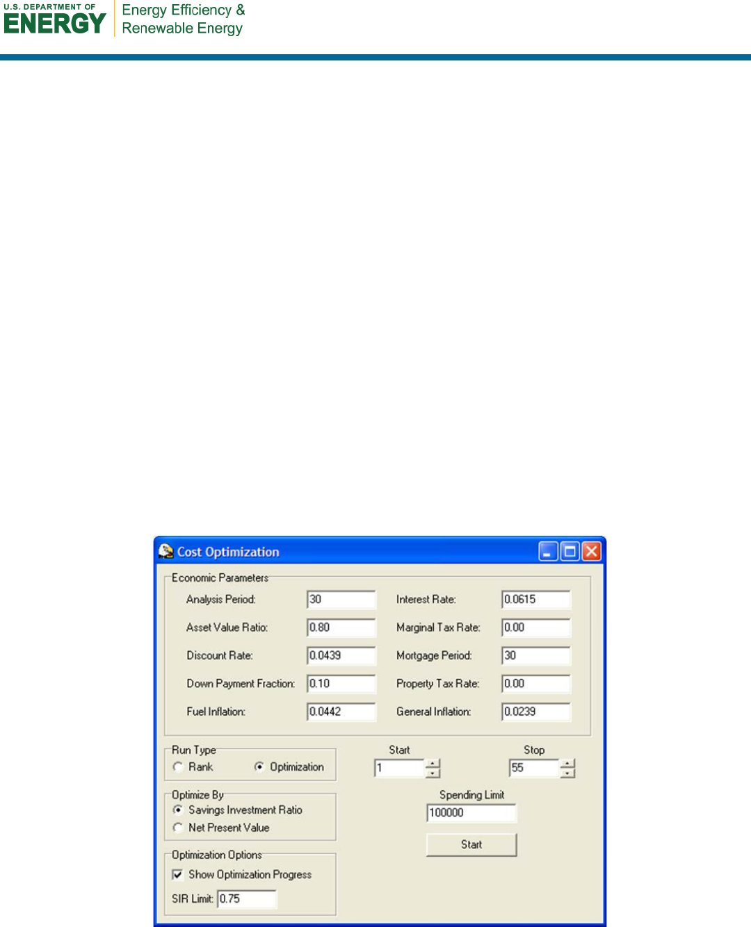
Optimization is initiated with the economic parameter and optimization control screen shown in
Figure 4. Unless otherwise stated, the values shown on this screen are those used for the
optimization analysis reported in this investigation. There are two notable exceptions:
• The mortgage period was set to 7 years for a selection of evaluations to study the impact
of this important economic variable.
• For at least one set of optimizations the interest rate was changed to 4% to reflect rates
that are available currently as a refinance (ReFi) option.
Figure 4. Starting screen for CostOpt

23
The Cost Optimization screen allows users to control the economic parameters as well as other
factors affecting the analysis. The Run Type option allows either a simple rank ordering of the
measures or a full optimization to be run. The Spending Limit will stop the optimization when
the specified expenditure limit has been reached. Optimization iterations can be ranked by either
SIR or NPV; NPV usually produces significantly fewer total simulations. An SIR limit can be
set, whereby only measures that exceed this limit are accepted. CostOpt also simulates solar
electric PV systems (Menicucci and Fernandez 1988).
8
If a PV system is included in the list of
measures to be considered, CostOpt will automatically set the optimization SIR Limit to either
the value entered on the startup screen or to the SIR for the PV system, whichever is less. A 5-
kWp
(dc)
PV system was included in all optimizations conducted for this investigation to
investigate geographic and economic impacts of its competition with efficiency improvements.
8
PVFORM, developed by Sandia National Laboratory, is used for PV simulations.
24
9 Results
9.1 Archetype Baseline Energy
How well the baseline energy consumption represents the housing stock is relevant to the
investigation. The U.S. EIA Residential Energy Consumption Survey (RECS) database provides
detailed microdata for the four largest states that can be used for this purpose. Table 8 presents a
comparison of the archetype baseline energy uses with the 2005 RECS data in these large states.
Table 8. Comparison of Baseline Home Energy Uses With 2005 RECS Data
New York Baseline Homes
2005 RECS Data
Mixed Fuel Homes
Simulation
Proto
error
Mean
StDev
n
kWh
8,364
–1.19%
8,465
5,331
47
Therms
1,180
3.78%
1,137
452
47
All-Electric Homes
kWh
n/a
n/a
n/a
n/a
n/a
California Baseline Homes
2005 RECS Data
Mixed Fuel Homes
Simulation
Proto
error
Mean
StDev
n
kWh
6,306
–
21.88%
8,072
5,153
217
Therms
418
–
26.76%
570
335
217
All-Electric Homes
kWh
11,290
–
19.24%
13,980
7,323
13
Texas Baseline Homes
2005 RECS Data
Mixed Fuel Homes
Simulation
Mean
StDev
n
kWh
12,282
–
21.13%
15,572
9,183
109
Therms
500
–0.71%
504
257
109
All-Electric Homes
kWh
18,830
–0.80%
18,981
7,127
56
Florida Baseline Homes
2005 RECS Data
Mixed Fuel Homes
Simulation
Proto
error
Mean
StDev
n
kWh
n/a
n/a
n/a
n/a
n/a
Therms
n/a
n/a
n/a
n/a
n/a
All-Electric Homes
kWh
17,651
–2.86%
18,171
6,890
86
Generally agreement was fairly good given the geographically coarse nature of the RECS data.
State RECS data are available for only the four most populous states, so these data do not
provide comparison for the other climates included in this investigation or for the specific
simulated locations—particularly important for a state such as California, where local climates
vary significantly. Thus, the fact that the archetype energy uses are from 4% larger to 26%

25
smaller than the mean values derived from the RECS data is not particularly problematic. The
fact that the archetype energy uses are smaller than the RECS averages probably tends to bias
optimization results toward conservative energy savings estimates.
Fourteen cities with a representative range of U.S. climates were included (hot humid, mixed,
cold, and marine) in the investigation. However, some cities have multiple archetype
expressions. For example, climate zone 2 has a significant number of homes with concrete
masonry wall systems and many with wood frame wall systems. Multiple space and water
heating fuels were often considered in many locations as commonly encountered. Thus, 22
archetypes were created in the 14 cities investigated, such that differing common alternatives
could be evaluated.
All-electric and mixed-fuel archetypes were created in a number of cities, and the optimization
analysis for each archetype allowed these fuels to be switched when the cost effectiveness
economics favored such a change.
Table 9 presents the baseline energy uses and costs for each archetype configuration. Source
energy use was calculated using the Building America fuel multipliers of 3.365 for electricity use
and 1.092 for natural gas use. Baseline source energy use across all archetypes varied from a
high of 247 MBtu for the concrete masonry wall archetype home with a heat pump and electric
water heating in Phoenix, Arizona to a low of 102 MBtu for the frame wall archetype home with
gas furnace and gas water heating in Los Angeles, California.
26
Table 9. Archetype Descriptions, Locations, and Baseline Energy Uses and Costs
Prototype Building
Description
Location
Cooling
Heating
Hot Water
L&A
Total
Total
Cost
City CZ kWh kWh Therms kWh Therms kWh kWh Therms
Source
MBtu
$/year
1600sf-1sty-SOG-CMU-HP
Miami
1
9,264
84
2,193
6110
17,651
203
$2,021
1600sf-1sty-SOG-CMU-HP
Houston
2
5,904
2,827
2,615
6110
17,456
200
$2,025
1600sf-1sty-SOG-Frm-GF
Houston
2
6,077
156
241
152
6110
12,343
393
185
$1,870
1600sf-1sty-SOG-Frm-HP
Houston
2
6,048
2,839
2,615
6110
17,612
202
$2,042
1600sf-1sty-SOG-CMU-HP
Phoenix
2
12,000
1,146
2,257
6110
21,513
247
$2,359
1600sf-1sty-SOG-Frm-GF
Phoenix
2
11,298
57
86
132
6110
17,465
217
224
$2,272
1600sf-1sty-SOG-Frm-HP
Phoenix
2
10,945
947
2,256
6110
20,258
233
$2,261
1600sf-1sty-Crwl-Frm-HP
Atlanta
3
3,389
5,747
2,999
6110
18,245
210
$1,837
1600sf-1sty-Crwl-Frm-GF
Atlanta
3
3,337
299
480
173
6110
9,746
653
183
$2,003
1600sf-1sty-Crwl-Frm-HP
Ft Worth
3
5,826
5,270
2,842
6110
20,048
230
$2,327
1600sf-1sty-Crwl-Frm-GF
Ft Worth
3
5,824
286
442
165
6110
12,220
607
207
$2,095
1600sf-1sty-Crwl-Frm-GF
Los Angeles
3
45
70
111
173
6110
6,225
283
102
$1,209
1600sf-1sty-Crwl-Frm-HP
Los Angeles
3
115
853
2,985
6110
10,063
116
$1,483
1600sf-1sty-Crwl-Frm-GF
San Francisco
3
49
227
361
191
6110
6,386
552
134
$1,504
1600sf-1sty-Crwl-Frm-HP
San Francisco
3
62
3,045
3,300
6110
12,517
144
$1,846
1600sf-1sty-Crwl-Frm-GF
Baltimore
4
2,108
531
845
194
6110
8,749
1,038
214
$2,586
1600sf-1sty-Crwl-Frm-GF
New York
4
1,640
614
982
198
6110
8,364
1,180
225
$3,276
1600sf-1sty-Crwl-Frm-HP
Seattle
4
233
9,571
3,562
6110
19,476
224
$1,568
1600sf-1sty-Crwl-Frm-GF
Seattle
4
189
537
878
205
6110
6,836
1,083
197
$1,918
1600sf-1sty-Crwl-Frm-GF
St Louis
4
2,768
572
904
192
6110
9,450
1,096
228
$2,178
1600sf-1sty-Bsmt-Frm-GF
Denver
5
607
491
732
207
6110
7,208
939
185
$1,581
1600sf-1sty-Bsmt-Frm-GF
Detroit
5
733
629
938
211
6110
7,472
1,149
211
$2,271
1600sf-1sty-Bsmt-Frm-GF
Minneapolis
6
423
805
1187
225
6110
7,338
1,412
238
$2,051
Building Description Key:
1600sf: Square feet of conditioned space
1sty: One story
SOG: Slab-on-grade foundation
Crwl: Crawlspace foundation
Bsmt: Unconditioned, unfinished basement foundation
CMU: Concrete masonry wall system
Frm:
Frame wall system
HP:
Heat pump archetype (electric space and water heating)
GF:
Gas furnace archetype (natural gas space and water heating)
CZ:
IECC Climate Zone

27
The annual energy costs for the archetypes varied by climate severity, but also by local energy
costs. The lowest annual energy cost of $1,209 was shown for the archetype in the mild weather
of Los Angeles, also with the lowest source energy use. By way of contrast, the archetype
located in the most severe cold climate, Minneapolis, Minnesota, had an annual energy cost of
$2,051. While the Minneapolis archetype’s source energy use was slightly greater than the New
York archetype, the annual energy cost for the New York archetype was $1,225 greater given the
much higher utility costs. Thus, while climate severity definitely made a significant difference to
source energy use, utility rates for electricity and natural gas had a much greater impact on
annual energy costs.

28
10 Cost Optimization Results
Four sets of optimization scenarios were conducted for this investigation, each with a different
scenario of financing assumptions and a relevant retrofit business model. The four scenarios are:
1. Default. A 30-year mortgage at 6.15% interest at full replacement cost
2. Homeowner finance. A 7-year mortgage at 6.15% interest at full replacement cost
3. HVAC contractor finance. A 7-year mortgage at 6.15% interest; incremental HVAC
costs
4. Remodel with refinancing. A refinanced 30-year mortgage at 4.0% interest rate at full
replacement costs.
The analysis period is 30 years for all four scenarios. Optimization Scenario 1 represents the
“default” economic cost-effectiveness optimization case as specified in Table 2 and in
accordance with the standards promulgated by RESNET (2012). Optimization Scenarios 2–4 are
designed to represent alternative business models or financing opportunities.
Optimization Scenario 2 represents the general home improvement model, where long-term
financing is unavailable and either a second mortgage or an unsecured loan is used to finance the
improvements over a 7-year term.
Optimization Scenario 3 represents the HVAC contractor business model, where long-term
financing is not available but the HVAC system has ceased to operate and must be replaced. For
Scenario 3, the cost of the replacement HVAC equipment is reduced to the incremental cost
difference between the minimum standard equipment and the improved efficiency equipment.
Optimization Scenario 4 represents the home mortgage refinance case where the homeowner or
homebuyer can take advantage of a reduced mortgage interest rate concurrent with a
comprehensive home energy improvement as part of a general house remodel.
10.1 Optimization Scenario 1
Optimization Scenario 1, the economic parameter default case, examines 23 archetypes in 14
cities comprising six IECC climate zones ranging from climate zone 1 to climate zone 6.
Summary results from this scenario of optimization runs are shown in Table 10. Six of the
archetypes shown in Optimization Scenario 1 were evaluated for this scenario only. These are
shaded light gray in Table 10. The remaining 17 archetypes were evaluated in each of the other
Optimization Scenarios. Standard CostOpt plots for each archetype are given in Appendix C.
These graphical results are useful in understanding the order in which improvement measures are
selected and their relative performance in reducing energy use and influencing homeowner
annual energy costs.
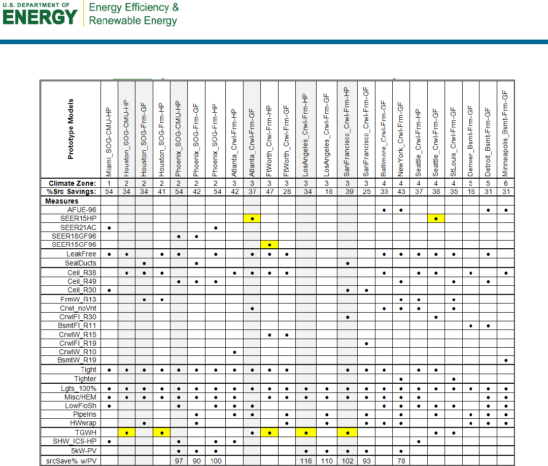
29
Table 10. Optimization Scenario 1—Default Economic Parameter
Optimizations
Seven instances of fuel switching are shown via yellow highlighting in Table 10. Five show fuel
switching from electricity to natural gas and two show switching from natural gas to electricity.
Fuel switching is largely attributed to water heating systems (five cases), where tankless gas
water heating systems are selected to replace electric hot water systems. However, one instance
(Ft. Worth) shows switching from electricity to natural gas for both the HVAC system and the
hot water system. And in Atlanta and Seattle we see HVAC fuel switching from a gas furnace to
an electric heat pump. Examination of the fuel costs provides ready explanation for these
choices. In Houston and Ft. Worth electricity is more than three times the cost of natural gas and
in Los Angeles and San Francisco electricity is more than four times the cost of natural gas. On
the other hand, in Atlanta and Seattle, where the fuel switching is in the opposite direction,
electricity is less than twice the cost of natural gas. In Baltimore, New York, Denver, Detroit,
and Minneapolis, we did not run all-electric cases as this is not common, so we do not see fuel
switching occurring in these climates even though it would not likely occur because electricity is
more than three times the cost of natural gas in these locations.

30
The two Phoenix all-electric cases are quite interesting. Electricity costs in Phoenix are less than
twice the cost of natural gas, but natural gas water heating is not selected for the all-electric
homes in Phoenix. Rather, because of the advantageous solar potential, a solar hot water system
is selected for both all-electric cases. Conversely, solar hot water is not selected in Phoenix for
the gas home archetype. Instead, the hot water pipes and the hot water tank are insulated—
measures that are not selected for the all-electric homes in Phoenix, where solar hot water
systems are selected instead.
This illustrates the importance of the relationship between electricity and gas prices to the
specific results. However, the absolute prices of gas and electricity are also very important to the
selection of improvement measures and the potential to cut source energy use through retrofit
measures. This is particularly true for PV, which is selected as cost effective in eight archetypes.
The five archetypes in California and New York all select 5-kW PV systems as cost effective
because of the high price of electricity in those states ($0.1475/kWh and $0.1874/kWh,
respectively). A 5-kW PV system is also selected as cost effective in Phoenix, where electricity
prices are much lower ($0.1097/kWh), but where the solar resource is the greatest of all the
climates studied. There, the generic 5-kW PV system produces 9,375 kWh/yr. In New York, San
Francisco, and Los Angeles, the 5-kW PV systems produce 6,971, 8,080, and 8,424 kWh/yr,
respectively. In New York, high electricity prices drive the selection of PV and in San Francisco
and Los Angeles, the combination of a good solar resource plus high electricity prices enhance
the desirability of the PV systems.
Utility prices also drive cost optimization from another important perspective. If utility prices are
low, fewer improvement measures are selected as cost effective and smaller savings percentages
are achieved. Denver, where electricity is $0.11/kWh and natural gas is $0.838/therm, offers
perhaps the best example of this fact. Denver has the lowest natural gas price of all 14 cities.
Thus, the cost-effective savings for the Denver natural gas archetype are only 18%, even though
the weather is fairly severe. In fact, because of the price of natural gas, it is not even cost
effective to improve the efficiency of the archetype 76% AFUE gas furnace in Denver,
something that was done in the other cold climate archetypes (Detroit and Minneapolis).
Table 10 also illustrates the sensitivity of improvement measures to their specific performance
and cost characteristics. For example, replacing 100% of the incandescent lighting with CFLs or
equivalent light-emitting diodes (LEDs) is cost effective in every location and circumstance.
Thus, this measure does not appear to be sensitive to either climate or utility price. Home energy
management (HEM) systems also appear to be cost effective across a large variety of climates
and archetypes. They are selected in all archetypes except four located in Atlanta, Seattle, St.
Louis, and Denver. Electricity prices are $0.10, $0.08, $0.09, and $0.11/kWh, respectively, in
these cities. We also see that for most climates, addressing duct leakage is cost effective. The
notable exceptions are Los Angeles, where the cooling and heating loads are very small, and in
most of the unconditioned basement archetypes, where the archetype distribution system leakage
is much less substantive.
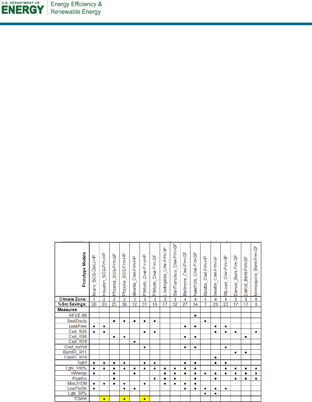
31
In 13 of the 23 archetypes, the hot water system is also improved. And in all cases where the hot
water system is not replaced, pipe insulation, hot water tank wrap, low-flow shower heads, or
some combination of these options are selected.
Ceiling insulation is also improved in all archetypes except those in Los Angeles, again
illustrating how benign this climate is with respect to heating and cooling loads. In fact, these
loads are so limited in Los Angeles that up to 34% source energy savings are achievable through
lighting, HEM, and water heating retrofits. However, this savings level is achievable only if the
archetype is all-electric. If the archetype has a gas space and water heating, only 18% efficiency
savings are cost effective. Against that limitation, however, >100% source energy savings are
cost effective in both Los Angeles archetypes with 5-kW PV systems that are indicated.
Optimization Scenario 1 achieves weighted average source energy savings or 37.4% without the
selected PV systems. If the five cases where PV is selected are included, the weighted average
source energy savings increase to 51.2%. Weighted average source energy savings are calculated
as the sum of the source energy savings for all archetypes divided by the sum of the base home
source energy use for all archetypes.
10.2 Optimization Scenario 2: Homeowner Financing
Optimization Scenario 2 is designed to study the cost effectiveness of a standard home
improvement mortgage, typically financed by the homeowner over a short 7-year period. A total
of 17 archetypes in 14 cities are evaluated. The mortgage period is set to 7 years and all other
economic parameter values are as in Scenario 1. The summary results are presented in Table 11.
Standard CostOpt plots for each archetype are given in Appendix D. These graphical results are
useful in understanding the order in which improvement measures are selected.
Table 11. Optimization Scenario 2—Home Improvement Mortgage Optimizations

32
The average source energy savings for these same archetypes in Optimization Scenario 1 is 36%.
For Optimization Scenario 2, the average is 21%—a 15% reduction in average source energy
savings from the reduced mortgage period. Reducing the mortgage term from 30 years to 7 years
means that monthly mortgage payments will be greater. This increase in short-term payments is
offset some by the fact that the analysis period remains 30 years and the energy cost benefits
continue to accrue after the mortgage is paid. However, the earlier and larger mortgage payments
result in less out-year discounting of the improvement costs while the future energy benefits are
discounted for the full period of the analysis. As a result, fewer measures are cost effective and
overall source energy savings are reduced.
Source energy savings of 30% are achievable in only three archetypes (Houston, Phoenix, and
New York) where tankless gas water heaters are cost effective. Two archetypes result in only
single-digit savings. The heat pump archetype in Seattle shows savings of only 7% and the
Minneapolis archetype shows savings of only 8%. This is explained by the fact that Seattle has
an electricity cost of only $0.08/kWh and Minneapolis has a gas cost of only $0.90/therm. Once
again, the strong influence of utility costs becomes evident in the level of improvements that can
be economically justified. For example, in New York where both electricity and natural gas costs
are relatively much greater ($0.18/kWh and $1.45/therm), the cost-effective energy savings are
34%.
The savings (and the installed measures) for Denver are almost identical for Optimization
Scenarios 1 and 2. The sole difference is that ceiling insulation goes to R-38 for Optimization
Scenario 1 but only R-30 for Optimization Scenario 2. Thus, again the very low cost of natural
gas in Colorado significantly reduces the cost effectiveness of improvement measures, nearly
irrespective of mortgage period.
Optimization Scenario 2 achieves weighted average source energy savings across all archetypes
and all climates of 21.5%. This is almost 16% less than the default scenario without PV and
almost 30% less than the default scenario with PV included in the average. The 5-kW PV system
is not cost effective for any location when the mortgage period is reduced to 7 years. On the
other hand, the 5-kW PV system proved cost effective for five archetypes when the mortgage
period was 30 years (Optimization Scenario 1).
10.3 Optimization Scenario 3: HVAC Contractor Financing
Many energy-using components in a home will eventually need replacement. A key ability of the
economic methods used in our evaluation has been to account for replacement—sometimes
multiple times—over the analysis time horizon. However, a less considered issue concerns how
components and equipment are considered that need replacement at the time, or very close to the
time, the retrofits are contemplated.
This circumstance is important because the incremental cost of choosing more efficient
equipment is often quite low at the time of replacement. For instance, in our base analysis, which
considers only outright replacement of functional equipment and components at full cost,
changing to a more efficient electric heat pump and more efficient windows will seldom be
selected in the optimization process. This is because replacing a working heat pump will often
cost $5,000 or more and replacing functional windows can cost easily cost twice that.

33
If the heat pump is no longer working and is at the end of its useful life, the incremental cost of
changing to a SEER-15/ HSPF-10 heat pump will often be only $500 after considering the $300
federal tax credit. The same is true for windows that need replacing, where the cost of replacing
standard double-glazed units with well-insulated, solar control low-e ones will only be a few
thousand dollars as opposed to $10,000 or more for outright replacement. On the other hand,
options such as PV systems or whole-house fans have incremental replacement costs that are the
same as those for outright replacement, because they are not otherwise necessary for a functional
household.
In the CostOpt analysis, it is possible to designate that certain items or equipment needs
replacement at the time of the retrofits. This causes the analysis to use the “incremental cost”
over the same less efficient minimum efficiency component to evaluate cost effectiveness. This
often results in options being selected that are otherwise not selected in the outright replacement
paradigm. Based on our evaluation, this often includes ENERGY STAR appliances, HVAC
systems, windows, changes to wall and roof color. These items are often cost effective, but only
at the time of natural replacement when a conventional replacement must be purchased anyway.
Figure 5 and Figure 6 reproduce two sets of optimization results for Ft. Worth, Texas. The
figures are in a standard CostOpt format that plots the cumulative investment costs and the
cumulative NPV of the investments on the left-hand vertical axis and the cumulative source
energy savings percentage on the right-hand axis. Thus, if an individual improvement measure
has an SIR greater than unity, cumulative NPV will increase. However, if an individual measure
has an SIR less than unity, cumulative NPV will decrease. Therefore, the point at which the NPV
is largest is the optimum cost effectiveness from the consumer’s perspective. However, measures
often come in at the end of the optimization that have an individual measure SIR less than unity
but that do not cause the cumulative NPV to drop below zero. These measures are also cost
effective from a societal perspective in that they are “paid for” by the earlier highly cost-
effective measures. Thus, the neutral cost point from the CostOpt perspective is the line where
the cumulative NPV equals zero. Because the optimization method is incremental, a number of
measures are selected and then later replaced by higher efficiency measures in the same
category. For ease of understanding, the final selections in each category are highlighted in light
green on the plots.
34
Figure 5. Ft. Worth analysis using full costs for all measures and outright replacement
Figure 6. Ft. Worth analysis using incremental costs (natural replacement costs) for all measures
Figure 5 shows results from the conventional “outright replacement” paradigm (Optimization
Scenario 1) where things are changed only if it is cost effective to pay full cost for removing and
replacing them with more efficient equipment and components. As the heat pump is still good,

35
its duct system is sealed and lighting is changed to CFLs or equivalent LEDs over the entire
home. Other parts of the building envelope are further improved—notably ceiling insulation goes
to R-38 and the crawlspace is sealed and insulated to R-15 on the exterior crawlspace walls.
Because of the cost advantage of natural gas in Texas, the optimization decides to replace the
standard electric water heater with a tankless gas model. The last installed measure with an SIR
greater than unity is the R-15 crawlspace wall insulation. At that point in the analysis, the NPV
of the improvements is maximized at $9,613 and an overall source energy savings of 32% is
achieved. This includes a reduction in electricity use of 7,514 kWh/yr and adds 115 therms/yr of
natural gas to cover water heating.
If the homeowner wants to install PV, the analysis indicates that other measures are cost
effective before that point—notably energy feedback with a HEM system, a fully condensing gas
furnace with a SEER-15 air conditioner, and leak-free ducts. The combination of all the
measures with a 5 kW PV system is able to bring the building to a net annual electricity use of
less than zero over the year (–188 kWh) and a source energy savings of 84%. The cumulative
package SIR to achieve a near zero energy building is slightly less than unity (0.964).
Figure 6 shows the results where all available items in the retrofit library are indicated as needing
replacement. The clothes washer and refrigerators are now cost effective to replace with
ENERGY STAR models and the heat pump is changed to a SEER-15 air conditioner with a 96%
efficient fully condensing natural gas furnace. The higher efficiency of the replaced HVAC
system has the impact of only justifying R-30 ceiling insulation and making the sealed
crawlspace with R-15 walls just outside the cost effectiveness limit (SIR = 1.0).
As before, fuel switching is also seen for water heating, where the optimization eventually
chooses a tankless gas water heater. Other observed differences include the call for replacing the
roofing with white shingles and choosing a light color for the house exterior walls when they
need repainting. Double-glazed, argon-filled low-e solar control windows are on the edge of cost
effectiveness when their replacement is required. Practically, this would be the indicated choice
for consumers needing to replace windows in Ft. Worth. A 41% source energy savings is
achieved at the last measure with an SIR greater than unity (tightening house leakage). This
comprises a reduction in electricity use of 12,478 kWh and adds 434 therms of natural gas use
for space and water heating.
The measures installed to this point of maximum cost effectiveness are sufficient to “pay for”
additional improvements before the “neutral cost point” for this home is reached. Figure 5 shows
that the 5-kW PV system drives NPV below zero; in Figure 6, the cost effectiveness of the
improvements (because they are all evaluated at their incremental cost rather than their full cost
of replacement) is large enough to “pay for” a number of additional improvement measures,
including the 5-kW PV system, still leaving a cumulative NPV for the cumulative improvement
investments of $10,176.
When the 5-kW PV system is added within the incremental analysis, three additional measures
are cost justified before PV: an unvented crawlspace, high efficiency windows and an energy

36
feedback system. Total annual electricity use is then –1,101 kWh and source energy savings over
the year are >87%.
9
A practical interpretation of the results of the incremental optimization in each location is that
while the outright replacement selection identifies robust measures that will always be included,
the incremental measures should be added to the package , if any of the chosen items in the
incremental analysis are in need of replacement at the time of retrofit.
For consumers, the results of the incremental optimization analysis indicates that even after the
retrofits are undertaken, the additional efficiency upgrade options indicated in the incremental
optimization should be considered to improve household efficiency over time as equipment and
components need replacement.
Generally the full incremental cost evaluation in higher electricity cost locations tended to call
for every means of reducing appliance electricity (particularly in cooling-dominated climates);
analysis in low-cost gas locations with gas appliances tends to justify lower potential savings
from selected retrofits.
One component of incremental cost analysis is of particular interest to this study—the
replacement of nonfunctioning HVAC systems. This is the focus of Optimization Scenario 3:
HVAC Contractor Financing. Optimization Scenario 3 is designed to study the cost effectiveness
of home improvements when the HVAC system requires replacement—the enlightened HVAC
contractor business model. HVAC systems have a useful lifetime of 12–18 years. Thus,
approximately 6% of all HVAC systems will be replaced each year. According to U.S. Census
data, there are approximately 82 million existing single-family homes. This means that
approximately 5 million HVAC replacements occur in American homes each year. From a
retrofit business model perspective, this represents a particularly intriguing opportunity to
influence energy efficiency decision making by homeowners. It is unlikely that the minimum
efficiency HVAC system will ever be the most cost-effective option for the homeowner when the
incremental cost of an upgrade is the economic cost effectiveness consideration. In addition, as
shown in Figure 6, such upgrades provide significant economic benefits that will effectively “pay
for” additional energy improvements to the home.
Seventeen archetypes in 14 cities are evaluated. The incremental cost of HVAC systems is used
in the analysis and the mortgage period is set to 7 years. All other economic parameter values are
as in Optimization Scenario 1. The summary results for Optimization Scenario 3 are presented in
Table 12. Standard CostOpt plots for each archetype are given in Appendix E. These graphical
results are useful in understanding the order in which improvement measures are selected.
9
This analysis does not consider utility pricing schemes for PV-powered homes that generate more than they use.
Some utilities will not pay anything for excess power produced annually beyond personal use. Others will pay the
customer for the power at the end of the year at the wholesale rate. A few will reimburse the homeowner at the retail
rate. Except in the latter case, an economically rational approach for the consumer would be to not change over
appliances to natural gas so that what would be an excess with gas appliances can be applied to reducing homeowner
costs to an absolute minimum. This can be accomplished simply in CostOpt by turning off the simulation flags that
allow fuel switching.
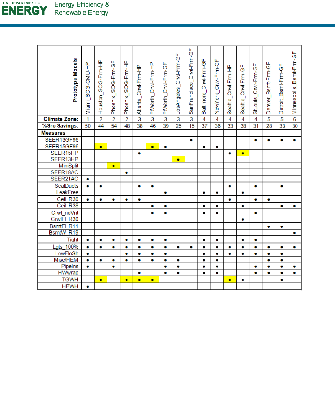
37
Table 12. Optimization Scenario 3—HVAC Replacement Optimizations
Table 12 clearly illustrates how incremental HVAC costs impact optimization results compared
with full HVAC costs. Save mild Los Angeles, every archetype installs an improved HVAC
system versus a minimum efficiency system. Fuel switching occurs from electric to gas space
heating in both Houston and Ft. Worth, where natural gas prices are relatively low compared to
electricity prices. Gas space heating switches to electric space heating in Seattle, where
electricity prices are relatively low compared to natural gas prices. There is also fuel switching
for tankless gas hot water systems where gas prices are advantageous.
10
A heat pump hot water
heater is selected only in Miami where gas was not available, although it would likely have been
chosen in other locations had there been a fixed cost associated with switching from electricity to
natural gas.
10
The identified level of fuel switching to gas may be lower in cases where gas service is not already available at the
home site as this cost is often $200–$500, depending on distances involved.
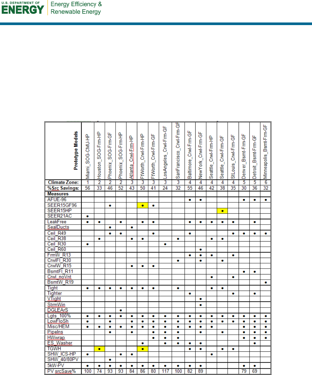
38
Weighted source energy savings for Optimization Scenario 3 are almost the same as for
Scenario 1. However, again if the 5-kW PV systems are included, Scenario 3 achieves 13.6%
less source energy savings than Scenario 1—again because a 7-year mortgage will not support
the relatively large first cost for the 5-kW PV system.
10.4 Optimization Scenario 4: Home Remodel Refinancing
Scenario 4 represents the home refinance model. The summary results for Optimization
Scenario 4 are presented in Table 13. Standard CostOpt plots for each archetype are given in
Appendix F. These graphical results are useful in understanding the order in which improvement
measures are selected.
Table 13. Optimization Scenario 4—Home Refinance Optimizations
Table 13 illustrates the much larger number of retrofit measures that qualify as cost effective
when the 30-year mortgage rate is reduced from 6.15% to 4.0%. Under the Remodel Refinance
39
scenario, the 5-kW PV system is cost effective in 13 of the 17 archetypes—eight more than
under Scenario 1. It is also apparent that the lower mortgage rate allows a larger fraction of high
first cost measures to qualify that did not qualify in Scenario 1. For example, HVAC systems are
improved in 10 archetypes under Scenario 4; only eight qualify under Scenario 1. High-cost
window replacements occur in two archetypes under Scenario 4; none occur in Scenario 1.
Weighted average source energy savings for Scenario 4 are 74% (41.3% without PV systems).
This is 23% larger than Scenario 1 with PV included.
Table 14 summarizes the achieved weighted average source energy savings and average NPV for
each of the four Optimization Scenarios. Weighted averages are calculated by taking the sum of
the source energy savings for all 17 archetypes in the sample set and dividing by the sum of the
original source energy use for all 17 archetypes. Average NPV is the simple average, calculated
as the sum of all seventeen individual NPVs divided by 17. Some business models are shown to
be more productive than others.
Table 14. Weighted Average Source Energy Savings and
Average NPV for Four Optimization Scenarios
Optimization Scenario
Source Savings
NPV
Measures
Selected
Without
PV
With
PV
Without
PV
With
PV
Scenario 1: Default
37.4% 51.2% $5,463 $5,586 27
Scenario 2: Homeowner Finance
21.5%
–
$1,019
–
18
Scenario 3: HVAC Finance
37.6%
–
$3,853
–
23
Scenario 4: Remodel Refinance
41.3% 74.0% $6,631 $6,904 31
The smallest weighted average source energy savings and average NPV are achieved by
Scenario 2, the homeowner-financed improvement mortgage with a 7-year term. Likewise, the
largest weighted average source energy savings and average NPV are achieved by Scenario 4,
the home refinance model. Because PV is cost effective in a number of locations examined by
this study, weighted average source energy savings and average NPV are both increased when
PV savings are included in the averages. For Scenario 1, the inclusion of cost-effective PV
systems raises the weighted average source energy savings from 37.4% to 51.2%. And for the
remodel refinance scenario, the weighted average source energy savings climbs from 41.3% to
74%—a 33% increase. A similar pattern can be observed in the number of selected measures in
each scenario. The smallest number is selected for Scenario 2, where financing is poorest and the
largest number is selected for Scenario 4, where financing is optimized.
Examination of the source energy savings bins achieved in each Optimization Scenario provides
additional insight into the results. Figure 7 presents the achieved source energy savings
(excluding any PV savings) for the 17 archetypes common to all Optimization Scenarios in the
study. This figure shows that homeowner financing (Scenario 2) offers the smallest potential for
cost effective home improvement with more than 75% of the archetypes achieving less than 30%
source energy savings. At the other extreme, the remodel/refinance (Scenario 4) usually produces
>30% source energy savings. The largest fraction of deep retrofit savings are also achieved
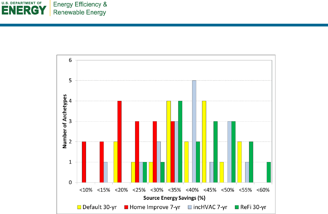
40
through the home refinancing in Scenario 4 with average savings of 74% (41% if PV is
excluded) ( a 5-kW PV system was cost effective in 13 of the 17 archetypes).
Figure 7. Source energy savings bins for the four optimization scenarios
A summary of the findings relative to specific measures and how they perform across climates,
utility costs, and financing scenarios follows:
• What works everywhere. CFLs, duct sealing, ceiling insulation, hot water tank wraps,
low-flow fixtures.
• What works in some places. Frame wall insulation, crawlspace wall insulation, solar
water heating, heat pump water heaters, PV systems, appliances that need replacement
and have low incremental costs.
• What does not work anywhere. Outright replacement of windows; most expensive
HVAC systems, and roof replacement.
10.5 Method in Action: Optimization Results for a Specific Home
In real-world use, the retrofit optimization method would not use averages, but specifics for an
individual house. This would include the pre-existing insulation and construction specifics,
relevant appliances and equipment efficiencies, and a list of the appliances and equipment in
likely need of replacement. House-specific thermostat preference and water consumption
intensity should likely be considered. Further, the specific utility costs and financing
arrangements would need to be realistically applied.
To illustrate how the described method would work in application, we show a case where a home
is audited in order to be retrofitted based on its particular situation. This home is exactly the
same as the standard building used in our analysis, but a number of differences are used to

41
illustrate how the starting efficiency and equipment, utility rates, and replacement status can
influence results. We used the default financing arrangements that are appropriate to a 30-year
re-mortgage associated with a remodeling effort, coordinated by an HVAC contractor to replace
an aging electric heat pump. The HVAC contractor works with auditors to perform a top-to-
bottom evaluation of the home’s energy upgrade needs and then recommends a comprehensive
series of measures targeted for the specific circumstances.
In our scenario, the home has just been purchased by a family of four in Ft. Worth, Texas. The
home has no natural gas access, the providing utility is TXU Energy, and the residential
electricity rate is $0.134/kWh. The home is 1974 vintage with a dark gray exterior. It needs
painting; the windows are leaking and need to be replaced. There are dense shade trees on the
east and west sides. The frame walls have no insulation, but there is R-19 blown insulation in the
attic. The crawlspace floors have no insulation. The heat pump needing replacement is assumed
to have an equivalent SEER of 9 Btu/Wh, although the owners had a utility duct sealing program
performed with the measured leakage to represent of Qn of 0.05. The new homeowners aim to
replace the heat pump and the aging dishwasher, and to purchase a new washing machine. The
household likes cool inside temperatures: 75°F in summer and 65°F in winter. The electric
resistance hot water tank is 10 years old and has an EF of 0.86. This family has two teenagers, so
the tank is set to 130°F to accommodate a large amount of hot water used each day (60 gal). The
original 25-ft
3
side-by-side refrigerator was audited and measured to use more than 4 kWh/day.
In the analysis, the equipment, settings, and insulation levels were adjusted and the following
items on the upgrade list were set to have incremental replacement costs: heating and air
conditioning, windows, dishwasher, clothes washer, and house paint. All natural gas options
were eliminated because access was lacking, and the prevailing utility costs were input. The
chosen objective for the home was to reach zero net annual source energy given the inputs.
Figure 8 shows that the specification of high higher utility rates and the incremental costs for
some measures have a dramatic impact on measure selection. The no-cost choice of a lighter
exterior color is made first; a SEER 15 heat pump and ENERGY STAR washer and dishwasher
soon follow. Low-e double glazed windows with argon fill are then selected. Some measures,
such as CFLs, airtightness, and ceiling insulation, are always chosen, although higher levels of
ceiling insulation are called for. Wall and floor insulation is selected for the uninsulated parts of
the structure and an ENERGY STAR refrigerator is specified along with an ICS solar water
heater supplying a heat pump water heater. Interestingly, the last measure selected was to change
the ducted central system for room-based mini-split heat pumps to eliminate duct losses.
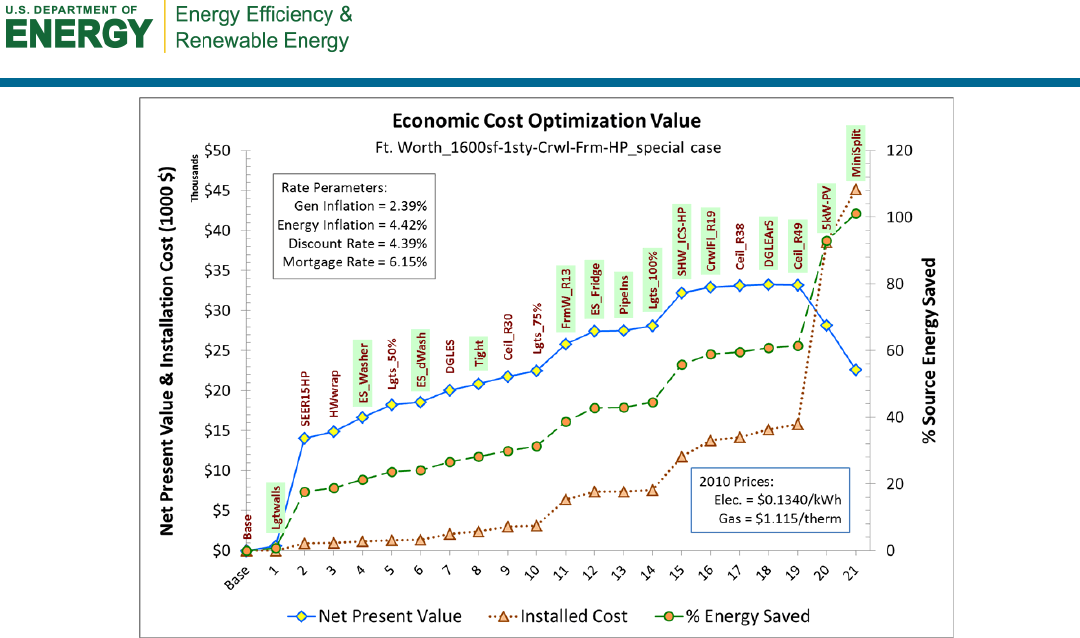
42
Figure 8. Optimization results for a specific home in Ft. Worth, Texas
The indicated source energy savings were just over 100% at an installed cost of $45,000 and a
first-year energy savings of $3,100. Even considering the added mortgage, the homeowners still
save $200/yr. The combination of higher utility prices, a more intensive use of cooling and hot
water, and replacement pricing for some options allows a greater justified level of energy
savings. The example also illustrates how modeling specific circumstances allows for a rational
method of selecting retrofit measures for specific homes.

43
11 Conclusions
We describe the results of using a comprehensive cost optimization model (EnergyGauge
CostOpt) across a range of representative climates in the United States. Similar to BEopt, the
model uses an iterative evaluation of all available measures, selecting the best performing option
before then reassessing all remaining options for future selection. The optimization process
typically takes 300–500 simulations before reaching the best performing package of 6–20 retrofit
measures that are most cost effective.
The purpose of the exercise was to critically evaluate a large library of potential retrofit options
with representative costs and performance and examine the various influences on potentials to
cost-effectively reduce energy use in existing U.S. housing. The predicted energy uses of
developed archetypes for the 14 locations simulated were favorably indexed where possible to
available RECS data. For the most part, cost data came from the NREL National Residential
Efficiencies Database, although augmented for estimating HVAC costs and those for renewable
energy systems. Energy costs were the revenue-based EIA utility averages in each state,
averaging $0.115/kWh and $1.174/therm. These are considered conservative in that they are now
two years old and do not include relevant utility state, local, and municipality taxes that are often
5%–15% greater than the EIA based numbers. The evaluation was carried out over a 30-year
time horizon with documented economic parameters used for the assessment.
BA-PIRC evaluated measures appropriate to addressing poorly insulated and equipped housing
stock 20 years or older. This located greatest opportunities, but the same approach can apply to
newer existing housing, although with often many fewer options chosen. Thus, the starting point
for an individual home will be important to its realistic savings potential. Still, many homes will
also be worse than the average starting point such that the savings potentials will remain very
large.
A key finding was that the energy efficiency levels of even older, inefficient homes can be
dramatically improved such that they can reach performance levels associated with zero energy
homes when evaluated on an annual source energy basis.
The results shown in the report can be considered conservative given that a small error in the P2
parameter was discovered at the end of report preparation which would tend to improve the cost-
effectiveness results for options with no maintenance and a long service life (e.g., insulation).
Also, two recent major studies (Hohen et al. 2011; Kok and Kahn 2012) reveal that the real
estate valuation of efficiency and PV measures is much higher than anticipated (approaching
90% of the investment cost at 5 year resale). Addressing this in the established economic
structure would entail reducing the rate at which resale/salvage values are discounted. This will
tend to improve cost effectiveness determinations, particularly for short-term financing. We
propose that the report eventually be reissued with the P2 error addressed as well as further
evaluation of the sensitivity to the rate of discounting of the salvage/resale value.
Source energy savings were greatest for the most extreme climates, but chosen measures were
very sensitive to measure cost and to prevailing utility costs. Where multiple fuels were
considered, some fuel switching was observed where the ratios of natural gas to electricity costs

44
were favorable. The analysis found a series of generic measures that were cost effective in nearly
all locations (such as greater ceiling insulation, lighting, low-cost hot water measures, and duct
sealing), whereas other options such as wall insulation and high-efficiency hot water systems
depend on relative climate severity and/or utility costs.
A number of measures (such as all ENERGY STAR appliances) were highly cost effective, but
only at the time of natural replacement. Some measures, such as high performance windows,
were cost effective only in the most severe climates. This finding indicates that in a real program,
the audited performance of each home, along with the remaining life of appliances and
equipment, and operational related characteristics could be favorably used with a tool such as
CostOpt to tailor a series of measures that are appropriate for that case so maximum savings are
achieved in the most cost-effective manner possible.
Relative to results from the optimization analysis, the highest nonrenewable energy savings were
achieved in hotter locations where more expensive electricity is used for cooling and potential
savings are large. Across locations, the lowest achievable savings tended to be in milder
climates, but in particular in locations with low natural gas prices.
The average achieved optimization savings were highly sensitive to the financing scheme and
interest rates used to pay for the retrofits. Using the default 6.15% financing over a 30-year
period, 51% source energy savings were indicated when including PV. Excluding PV, the
savings were 37%, indicating the increasing relevance to solar electric generation to the retrofit
approach now available.
Financing schemes were quite important—a fact with direct relevance to policy decisions
relative to energy savings programs for existing U.S. housing. Homeowner-financed energy
retrofits failed to achieve average savings >21% because of the higher annual costs incurred by
the short finance period.
A financing model where retrofits are installed along with replacement of the HVAC system was
superior to homeowner financing. In this scenario, the incremental HVAC costs were applicable,
resulting in higher achieved source energy savings (37%), although many potential measures
with high savings are still ignored because of the short financing terms.
The greatest energy savings—averaging 74% when PV was included—were based on a 30-year
home remodel/refinancing scheme for which the interest rate was 4%. Programmatically, such a
program might focus on home remodeling and refinancing and/or on the same at the time of
resale. Another possibility would be to improve homes in the foreclosure market prior to resale.
Interestingly, this scenario showed solar electricity to be cost effective or near cost effective in
most U.S. locations at $6.50/W installed. At a cost of $5/W installed, such systems would be cost
effective across the United States, as long as the federal tax credit remains applicable. In
particular, the results of the home refinance scenario results indicated that near zero source
energy (>80% savings) was cost effective in eight of the 14 U.S. climates. These tended to be
those with sunnier conditions and higher applicable electricity prices.

45
Observing the very large identified energy savings in older housing stock in the United States,
implementation concerns become central—particularly given the lack of homeowner knowledge
and motivation. Accordingly, the results suggest that:
• Efforts should be made to create a national retrofit program that seeks to match long-term
financing with multiple retrofit options that are effectively bundled together.
• Program participation could be matched to replacement of major HVAC system or hot
water system improvements. These could be contracted at once with tailored retrofit
measures chosen by a customized computerized evaluation that considers the starting
point of home features and equipment along with local utility pricing.
• Participating households should have an evaluation of appliance age and functionality to
take advantage of cost-effective opportunities for appliance replacement during the
retrofit process.

46
References
Casey, S.; Booten C. (2011). Energy Savings Measure Packages: Existing Homes. Golden, CO:
National Renewable Energy Laboratory. NREL/TP-5500-53023.
www.nrel.gov/docs/fy12osti/53023.pdf.
Christensen, C.; Anderson, R. Horowitz, S; Courtney A.; Spencer, J. (2006). BEopt Software for
Building Energy Optimization: Features and Capabilities. Golden, CO: National Renewable
Energy Laboratory. NREL/TP-550-39929. www.nrel.gov/buildings/pdfs/39929.pdf.
Duffie, J.A.; Beckman, W.A. (1980). Solar Engineering of Thermal Processes, pp. 381-406,
New York: John Wylie & Sons, Inc.
Hendron, R. (2006). Building America Performance Analysis Procedures for Existing Homes.
Golden, CO: National Renewable Energy Laboratory. NREL/TP-550-38238.
http://www.nrel.gov/docs/fy06osti/38238.pdf
Hohen, B.; Wisser, R.; Cappers, P.; Thayer, M. (2011). An Analysis of the Effects of Residential
Photovoltaic Energy Systems on Home Sales Prices in the California Market, Berkeley, CA:
Lawrence Berkeley National Laboratory, LBNL-4476e, April 2011.
Kok, N.; Kahn, M.E. (2012). The Value of Green Labels in the California Housing Market, UC
Berkeley and UCLA.
McIlvaine, J.R. (2011). “NREL Submission Work,” unpublished test results spreadsheet and
email to D. Parker, dated 9 June 2011.
Menicucci, D.F.; Fernandez, J.P. (1988). User’s Manual for PVFORM: A Photovoltaic System
Simulation Program for Stand-Alone and Grid-interactive Applications. Albuquerque, NM:
Sandia National Laboratories. Report 85-0375.
http://prod.sandia.gov/techlib/access-
control.cgi/1985/850376.pdf.
Parker, D.; Huang, Y.; Konopacki, S.; Gartland, L.; Sherwin J.; Gu, L. (1998). “Measured and
Simulated Performance of Reflective Roofing Systems in Residential Buildings.” ASHRAE
Transactions, Vol. 104, Pt. 1, Atlanta, GA: American Society of Heating, Refrigerating and Air
Conditioning Engineers.
Pigg, S.; Francisco, P. (2006). A Field Study of Exterior Duct Leakage in New Wisconsin
Homes, ECW.
Polly, B.; Gestwick, M.; Bianchi, M.; Anderson, R.; Horowitz, S.; Christensen, C.; Judkoff, R.
(2011). Method for Determining Optimal Residential Energy Efficiency Retrofit Packages.
Golden, CO: National Renewable Energy Laboratory. TP-5500-50572; DOE/GO-102011-3261.
www.nrel.gov/docs/fy11osti/50572.pdf.
RESNET. (2012). Mortgage Industry National Home Energy Rating Systems Standards, Section
303.3.3 Economic Cost Effectiveness. Oceanside, CA: Residential Energy Services Network.
www.resnet.us/standards/mortgage.

47
Sherman, M.H.; Wilson, D.J.; Kiel, D.E. (1986). “Variability in Residential Air Leakage,” in
Measured Air Leakage in Buildings, ASTM Special Publication 904, Philadelphia, PA.
Walker, I.S. (1998). Technical Background for Default Values used for Forced Air Systems in
Proposed ASHRAE standard 152P. ASHRAE Trans. Vol.104 Part 1. Presented at ASHRAE TC
6.3 Symposium, January 1998. LBNL 40588.

48
Appendix A. Calculation of Economic Cost Effectiveness
Section of RESNET Standards
303.3.3 Economic Cost Effectiveness. If ratings are conducted to evaluate energy
saving improvements to the home for the purpose of an energy improvement
loan or energy efficient mortgage, indicators of economic cost effectiveness shall
use present value costs and benefits, which shall be calculated as follows:
LCC
E
= P1*(1
st
Year Energy Costs) (Eq 303.3.3-1)
LCC
I
= P2*(1
st
Cost of Improvements) (Eq 303.3.3-2)
where:
LCC
E
= Present Value Life Cycle Cost of Energy
LCC
I
= Present Value Life Cycle Cost of Improvements
P1 = Ratio of Life Cycle energy costs to the 1
st
year energy costs
P2 = Ratio of Life Cycle Improvement costs to the first cost of improvements
Present value life cycle energy cost savings shall be calculated as follows:
LCC
S
= LCC
E,b
– LCC
E,i
(Eq 303.3.3-3)
where:
LCC
S
= Present Value Life Cycle Energy Cost Savings
LCC
E,b
= Present Value LCC of energy for baseline home configuration
LCC
E,i
= Present Value LCC of energy for improved home configuration
Standard economic cost effectiveness indicators shall be calculated as follows:
SIR = (LCC
S
) / (LCC
I
) (Eq 303.3.3-4)
NPV = LCC
S
- LCC
I
(Eq 303.3.3-5)
where:
SIR = Present Value Savings to Investment Ratio
NPV = Net Present Value of Improvements
303.3.3.1 Calculation of P1 and P2. The ratios represented by P1 and P2 shall be calculated
in accordance with the following methodology
11
:
P1 = 1/(DR-ER)*(1-((1+ER)/(1+DR))^nAP) (Eq 303.3.3-6a)
or if DR = ER then
P1 = nAP / (1+DR) (Eq 303.3.3-6b)
11
Duffie, J.A. and W.A. Beckman, 1980. Solar Engineering of Thermal Processes, pp. 381-406, John Wylie &
Sons, Inc., New York, NY.

49
where:
P1 = Ratio of Present Value Life Cycle Energy Costs to the 1
st
year Energy Costs
DR = Discount Rate as prescribed in section 303.3.3.2
ER = Energy Inflation Rate as prescribed in section 303.3.3.2
nAP = number of years in Analysis Period as prescribed in section 303.3.3.2
P2 = DnPmt + P2
A
+ P2
B
+ P2
C
- P2
D
(Eq 303.3.3-7)
where:
P2 = Ratio of Life Cycle Improvement costs to the first cost of improvements
DnPmt = Mortgage down payment rate as prescribed in section 303.3.3.2
P2
A
= Mortgage cost parameter
P2
B
= Operation & Maintenance cost parameter
P2
C
= Replacement cost parameter
P2
D
= Salvage value cost parameter
P2
A
= (1-DnPmt)*(PWFd/PWFi) (Eq 303.3.3-8a)
where:
PWFd = Present Worth Factor for the discount rate = 1/DR*(1-(1/(1+DR)^nAP))
PWFi = Present Worth Factor for the mortgage rate = 1/MR*(1-(1/(1+MR)^nMP))
DR = Discount Rate as prescribed in section 303.3.3.2
MR = Mortgage interest Rate as prescribed in section 303.3.3.2
nAP = number of years of the Analysis Period as prescribed in section 303.3.3.2
nMP = number of years of the Mortgage Period
P2
B
= MFrac*PWinf (Eq 303.3.3-8b)
where:
MFrac = annual O&M costs as a fraction of first cost of improvements
12
PWinf = ratio of present worth discount rate to present worth general inflation rate
= 1/(DR-GR)*(1-(((1+GR)/(1+DR))^nAP))
or if DR = GR then
= nAP/(1+DR)
GR = General Inflation Rate as prescribed in section 303.3.3.2
P2
C
= Sum {1/((1+(DR-GR))^(Life*i))} for i=1, n (Eq 303.3.3-8c)
where:
i = the i
th
replacement of the improvement
12
The maintenance fraction includes all incremental costs over and above the operating and maintenance cost of the
“standard” measure. Where components of a system have various lifetimes, the longest lifetime may be used and the
components with shorter lifetimes may be included as a maintenance cost at the present value of their future
maintenance cost. The maintenance fraction may also be used to represent the degradation in performance of a given
system. For example, photovoltaic (PV) systems have a performance degradation of about 0.5% per year and this
value can be added to the maintenance fraction for PV systems to accurately represent this phenomenon in this cost
calculation procedure.

50
Life = the expected service life of the improvement
P2
D
= RLFrac / ((1+DR)^nAP)
13
(Eq 303.3.3-8d)
where:
RLFrac = Remaining Life Fraction following the end of the analysis period
303.3.3.2 Determination of Economic Parameters. The following economic parameter
values shall be determined by RESNET in accordance with this Section each January using the
latest available specified data and published on the RESNET website.
• General Inflation Rate (GR)
• Discount Rate (DR)
• Mortgage Interest Rate (MR)
• Down Payment Rate (DnPmt)
• Energy Inflation Rate (ER)
The economic parameter values used in the cost effectiveness calculations specified in Section
303.3.3.1 shall be determined as follows:
303.3.3.2.1 General Inflation Rate (GR) shall be the greater of the 5-year and the 10-year
Annual Compound Rate (ACR) of change in the Consumer Price Index for Urban Dwellers
(CPI-U) as reported by the U.S. Bureau of Labor Statistics,
14
where ACR shall be calculated as
follows:
ACR = ((endVal)/(startVal))^(1.0/((endYr)-(startYr)))-1.0 (Eq 303.3.3-9)
where:
ACR = Annual Compound Rate of change
endVal = Value of parameter at end of period
startVal = Value of parameter at start of period
endYr = Year number at end of period
startYr = Year number at start of period
303.3.3.2.2 Discount Rate (DR) shall be equal to the General Inflation Rate plus 2%.
303.3.3.2.3 Mortgage Interest Rate (MR) shall be defaulted to the greater of the 5-year and
the 10-year average of simple interest rate for fixed rate, 30-year mortgages computed from the
Primary Mortgage Market Survey (PMMS) as reported by Freddie Mac unless the mortgage
interest rate is specified by a program or mortgage lender, in which case the specified mortgage
13
Based on recent research by Kok and Kahn (2012) and Hohen et al. (2011), energy efficiency and PV system
improvements are strongly valued by the public at resale—up to 90% of original value at the time of resale at five
years. This would indicate that the salvage/resale value parameter should be only very lightly discounted—perhaps
half the conventional discount rate. Although this was not evaluated in this study, sensitivity might be investigated
in the future. In any case, not incorporating this real market influence represents conservatism in this study.
14
http://www.bls.gov/CPI/#tables

51
interest rate shall be used. The mortgage interest rate used in the cost effectiveness calculation
shall be disclosed in reporting results.
303.3.3.2.4 Down Payment Rate (DnPmt) shall be defaulted to 10% of 1
st
cost of
improvements unless the down payment rate is specified by a program or mortgage lender, in
which case the specified down payment rate shall be used. The down payment rate used in the
cost effectiveness calculation shall be disclosed in reporting results.
303.3.3.2.5 Energy Inflation Rate (ER) shall be the greater of the 5-year and the 10-year
Annual Compound Rate (ACR) of change in the Bureau of Labor Statistics, Table 3A, Housing,
Fuels and Utilities, Household Energy Index
15
as calculated using Equation 303.3.3-9.
303.3.3.2.6 Mortgage Period (nMP) shall be defaulted to 30 years unless a mortgage finance
period is specified by a program or mortgage lender, in which case the specified mortgage period
shall be used. The mortgage period used in the cost effectiveness calculation shall be disclosed in
reporting results.
303.3.3.2.7 Analysis Period (nAP) shall be 30 years.
303.3.3.2.8 Remaining Life Fraction (RLFrac) shall be calculated as follows:
RLFrac = (nAP/Life) – (Integer (nAP/Life)) Eqn. 303.3.3-10
or if Life > nAP
RLFrac = (Life-nAP) / nAP
where:
Life = useful service life of the improvement(s)
303.3.3.2.9 Improvement Costs. The improvement cost for Energy Conservation Measures
(ECMs) shall be included on the Economic Cost Effectiveness Report.
303.3.3.2.9.1 For New Homes the improvement costs shall be the full installed cost of the
improvement(s) less the full installed cost of the minimum standard or code option less any
financial incentives that accrue to the home purchaser.
303.3.3.2.9.2 For Existing Homes the improvement costs shall be the full installed cost of the
improvement(s) less any financial incentives that accrue to the home purchaser.
303.3.3.2.10 Measure Lifetimes. The ECM service life shall be included on the Economic Cost
Effectiveness Report. Appendix C of this standard provides informative guidelines for service
lifetimes of a number of general categories of ECMs.
303.3.3.3 The annual energy cost savings for the Rated home shall be estimated by comparing the
projected annual energy cost of the Rated home to the projected annual energy cost of a baseline
home. For new homes, the most recent HERS Reference home shall be the baseline, except when an
15
http://www.bls.gov/cpi/cpi_dr.htm
52
alternative reference home is specified by the lender or program underwriter. For existing homes, the
unimproved home shall be used as the baseline.
303.3.3.4 The estimated monthly energy cost savings for the Rated home shall be equal to the annual
energy cost savings divided by 12.
303.3.3.5 For FHA and Freddie Mac energy mortgages, the present value of energy savings
shall be calculated in accordance with Equation 303.3.3-3 where the baseline home is as
specified by the most current HUD Mortgage Letter.

53
Appendix B. Determination of HVAC Equipment Costs
NREL maintains a very useful online National Residential Efficiency Measure Database
(http://www.nrel.gov/ap/retrofits/index.cfm) containing estimated retrofit costs for HVAC
equipment.
The HVAC cost data are cast in terms of only the equipment capacity as Cost = a*CAP. The
database provides the value of ‘a’ for each listed efficiency. Although it would likely be possible
to use the listed efficiencies to develop a formulation cast in terms of both efficiency and
capacity (e.g. Cost = a*CAP + b*EFF), this likely does not adequately characterize costs.
Conventional pricing logic implies that fixed and variable costs are associated with HVAC
installation. This can be empirically verified by regressing on collected cost data where fixed and
variable cost components are clearly revealed. For example, fixed costs are associated with
selling the new equipment, dispatching a vehicle and service personnel to the installation site,
removing the old equipment, and hooking up the new equipment that are not tied directly to the
efficiency or the size of the new equipment. Thus, the characterization of HVAC costs as
stemming solely from equipment efficiency and capacity tends to underestimate costs for small
capacity equipment (which will incur a larger percentage of fixed costs relative to total cost) and
overstate costs for large capacity equipment (which will incur a smaller percentage of fixed costs
relative to total cost).
BA-PIRC attempted to characterize the fixed costs associated with HVAC replacements using an
empirical approach. Available online retail costs from available manufacturers were used to
determine the, uninstalled retail cost of a variety of HVAC equipment. One clear advantage of
this method is that the cost data, unlike those collected from installers are very consistent in their
origin with less statistical variation. To these online values were added fixed costs that make up
the total price similar to those observed in the NREL database. The resulting total cost data are
then regressed in terms of equipment efficiency and capacity for four categories of commonly
available HVAC equipment. The four categories are:
• Heat pumps
• Air conditioners (with strip resistance heating)
• Gas furnaces (with no air conditioning)
• Gas furnace-air conditioner combinations
For each equipment category, an 8% tax was applied to the online retail cost plus a fixed
“service” cost plus 35% overhead and profit, such that
Total Cost = Retail*1.08 + $750 + Retail*0.35
The fixed “service” cost is calculated based on 4 man-hours of sales time at $28.00 per hour and
16 hours of installation time at $22.50 per hour with a 10% fringe and 30% overhead added to
these salary rates. In addition, a daily average truck charge of $100 is added to this total salary
charge to arrive at the fixed service charge.
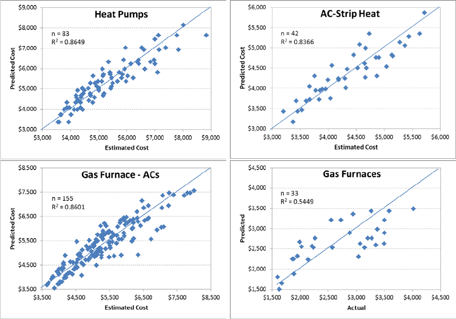
54
The resulting total cost estimates are then regressed against the equipment capacity and
efficiency from online data sources to arrive at generalized equations that can be used to
calculate the HVAC costs used in the CostOpt optimizations. The resulting equations are as
follows.
Heat Pumps: -5539 + 604*SEER + 699*tons
Air Conditioners (with strip heat): –1409 + 292*SEER + 520*tons
Gas Furnace/air conditioner: –6067 + 568*SEER + 517*tons + 4.04*kBtu + 1468*AFUE
Gas Furnace only: –3936 + 14.95*kBtu + 5865*AFUE
Results from the regressions showing the sample size (n) and correlation coefficient (R
2
) for each
equipment category are shown in Figure 9.
Figure 9. Results from regression analysis of CostOpt HVAC cost estimates
Considering the variability of the marketplace, the correlation coefficients are reasonable for
these regressions. For comparison, Tables 15 through Table 17 show the range of costs provided
by the NREL database for replacement heat pumps, air conditioners, and gas furnaces.

55
Table 15. NREL Cost Estimates for Heat Pumps
NREL Heat Pump Replacement Costs
SEER
Low
$/kBtu
High
$/kBtu
Average
$/kBtu
± %
13
97
170
140
26%
14
110
180
140
25%
15
110
190
150
27%
16
120
200
160
25%
17
130
210
170
24%
18
140
220
180
22%
19
140
230
180
25%
20
150
230
190
21%
21
160
240
200
20%
Table 16. NREL Cost Estimates for Air Conditioners
NREL Air Conditioner Replacement Costs
SEER
Low
$/kBtu
High
$/kBtu
Average
$/kBtu
± %
13
59
190
130
50%
14
66
200
130
52%
15
73
210
140
49%
16
80
210
150
43%
17
87
220
150
44%
18
94
230
160
43%
19
100
230
170
38%
20
110
240
170
38%
21
110
250
180
39%
Table 17. NREL Cost Estimates for Gas Furnaces
NREL Gas Furnace Replacement Costs
AFUE
Low
$/kBtu
High
$/kBtu
Average
$/kBtu
± %
78%
8.7
33.3
15
82%
80%
8.7
35.3
18
74%
82%
8.7
38.3
21
70%
90%
14.7
49.3
32
54%
92%
17.7
52.3
35
49%
94%
20.7
55.3
38
46%
96%
23.7
58.3
41
42%
These estimates indicate significant variations in the marketplace with respect to HVAC costs
and to a certain degree mirror the variations in costs represented in Figure 9, with gas furnaces
showing the largest variance.
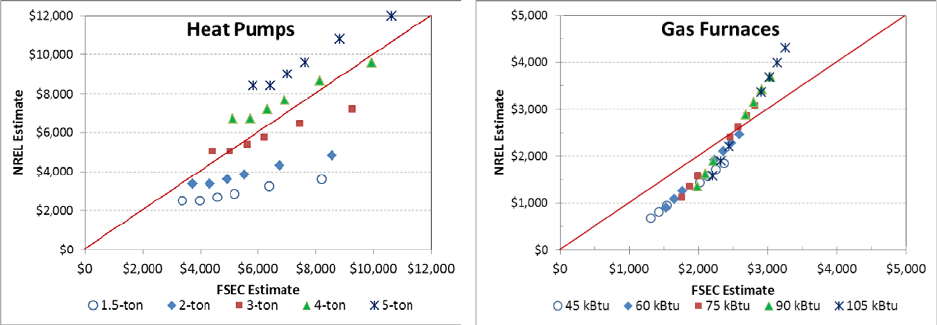
56
BA-PIRC evaluated the CostOpt estimates against those provided by the NREL database average
cost estimates for heat pumps and gas furnaces. Figure 10 presents the results of this comparison.
Figure 10. Comparison of CostOpt HVAC cost estimates and NREL HVAC cost estimates
In Figure 10 the individual plot points represent different efficiencies, with SEERs of 13, 14, 15,
16, 18, and 21 represented on the heat pump chart. The right-hand panel shows data for furnaces:
with representative AFUEs of 78%, 80%, 82%, 90%, 92%, 94%, and 96%. Each chart also
distinguishes between different capacities, with 1.5-, 2-, 3-, 4-, and 5-ton equipment on the heat
pump chart and 45, 60, 75, 90, and 105 kBtu/h equipment on the gas furnace chart.
Both charts show that the CostOpt estimates are larger for the lower capacity and smaller for the
larger capacity equipment. The charts also show that, on average, the CostOpt estimates are
consistent with the NREL estimates. However, the fact that the CostOpt estimates treat fixed
costs more explicitly is evident on both charts. In a practical sense, the CostOpt estimates
generally show that monetary savings in the capacity of installed equipment coming from more
efficient envelope measures are slightly less important than the original values in the NREL
database.
57
Appendix C. Optimization Scenario 1—
Default Economic Parameter Model
The figures shown on the following pages are in a standard CostOpt format that plots the
cumulative investment costs and the cumulative NPV of the investments on the left-hand vertical
axis and the cumulative source energy savings percentage on the right-hand axis. Thus, if an
individual improvement measure has an SIR greater than unity, cumulative NPV will increase.
However, if an individual measure has an SIR less than unity, cumulative NPV will decrease.
Therefore, the point at which the NPV is largest is the optimum cost effectiveness from the
consumer’s perspective. However, often measures come in at the end of the optimization that
have an individual measure SIR less than unity but that do not cause the cumulative NPV to drop
below zero. These measures are also cost effective from a societal perspective in that they are
“paid for” by the earlier highly cost-effective measures. Thus, the neutral cost point from the
CostOpt perspective is the line where the cumulative NPV equals zero. Because the optimization
method is incremental, a number of measures are selected and then later replaced by higher
efficiency measures in the same category. Thus, for ease of understanding, the final selections in
each category are highlighted in light green on the plots.
Key to acronyms:
1600sf: Archetype home size in square feet
1sty: One-story abov- grade home
SOG: Slab-on-grade foundation
Crwl: Crawlspace foundation
Bsmt: Unconditioned basement foundation
HP: Electric space and water heating in base archetype
GF: Natural gas space and water heating in base archetype
7-yr: Seven year mortgage period (used in Scenarios 2 and 3)
incHVAC: Incremental costs used for HVAC systems (used in Scenario 3)
ReFi: Refinance scenario using 4% mortgage interest (used in Scenario 4)
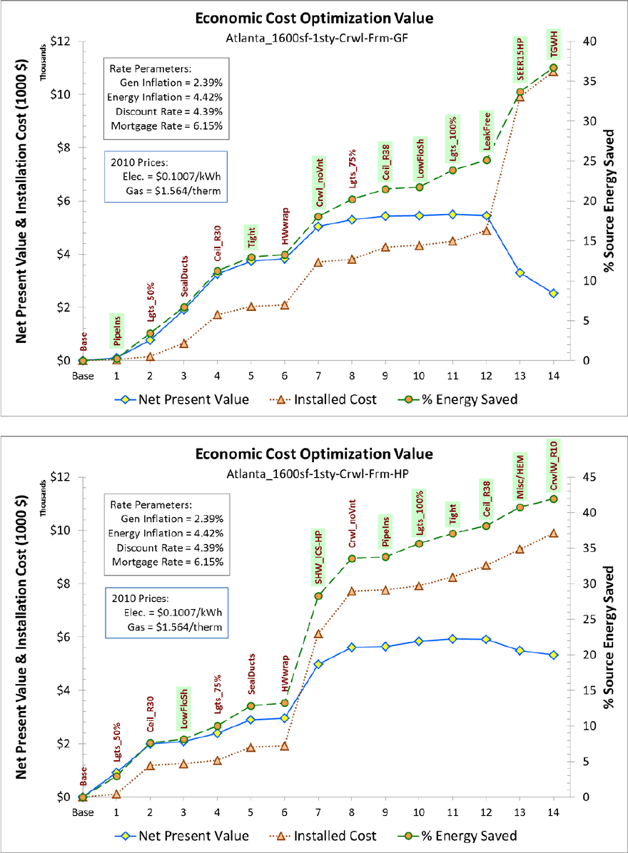
58
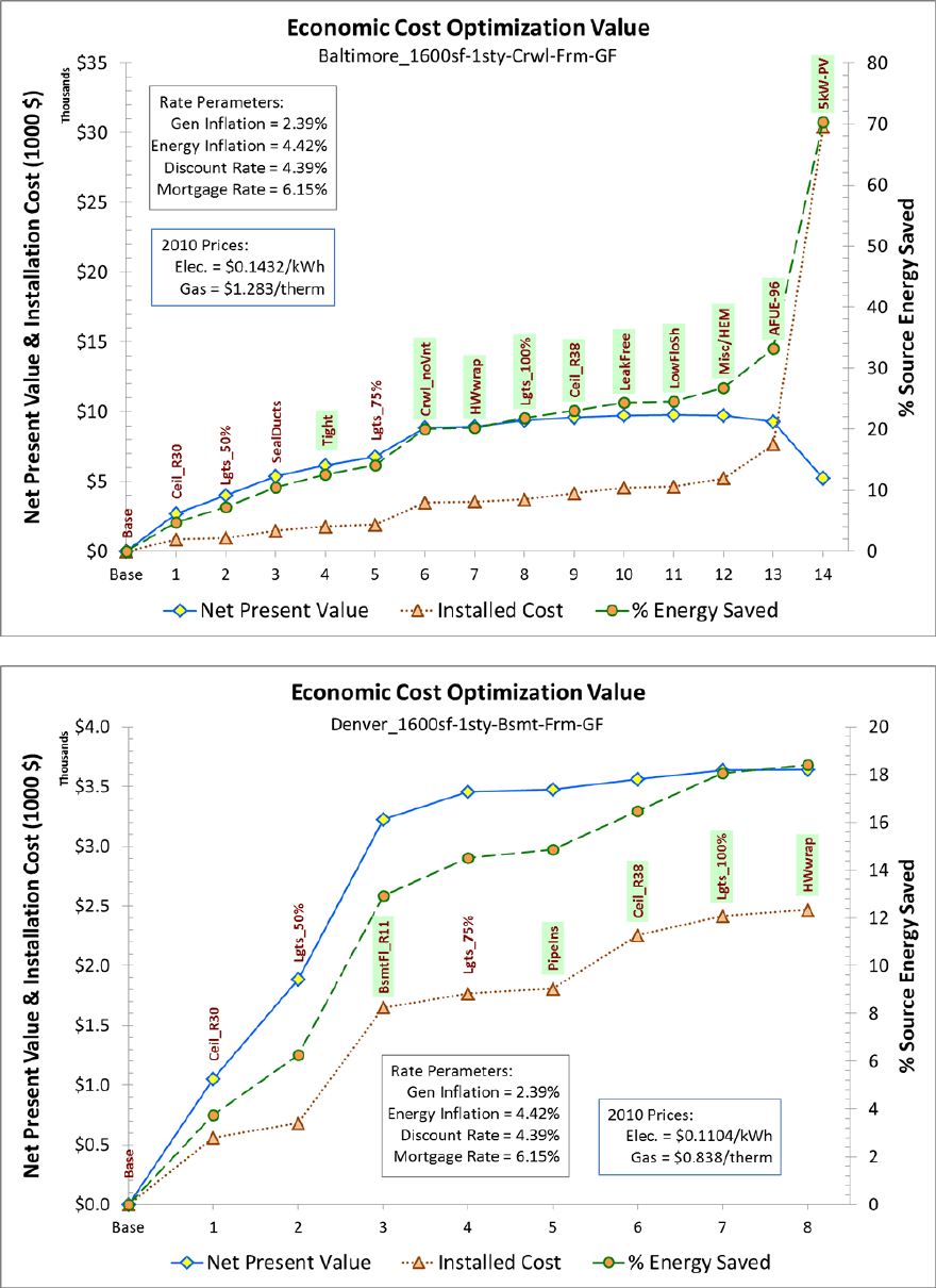
59
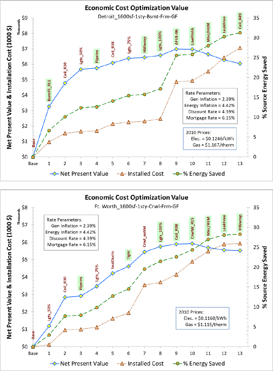
60
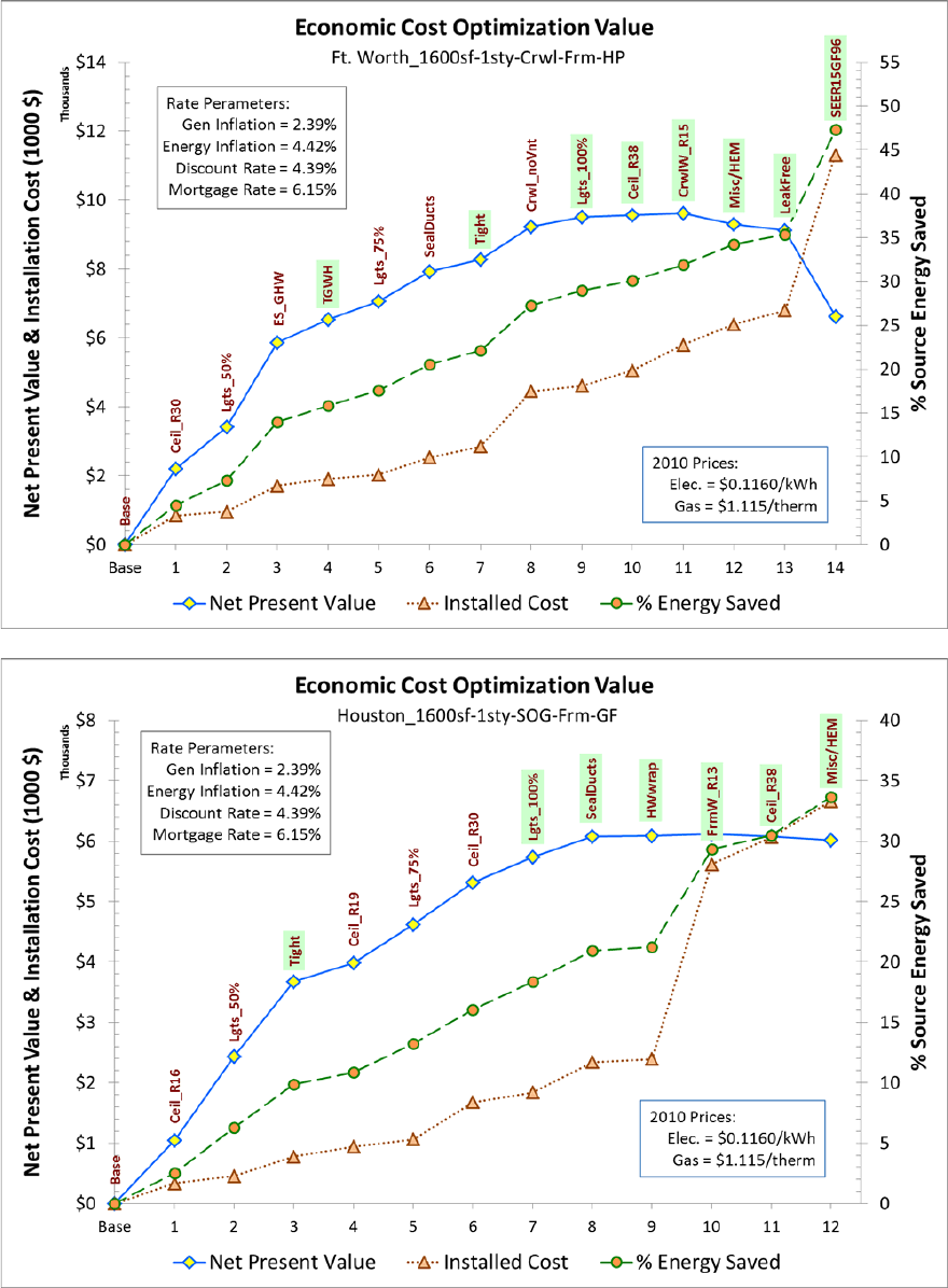
61
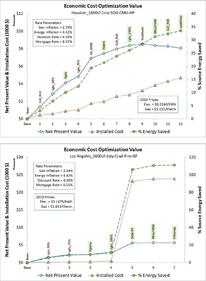
62
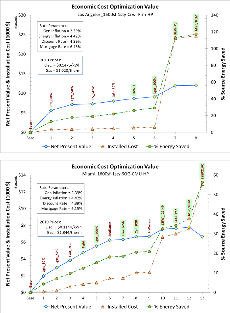
63
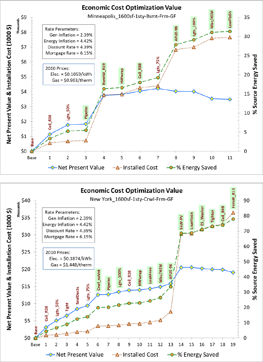
64
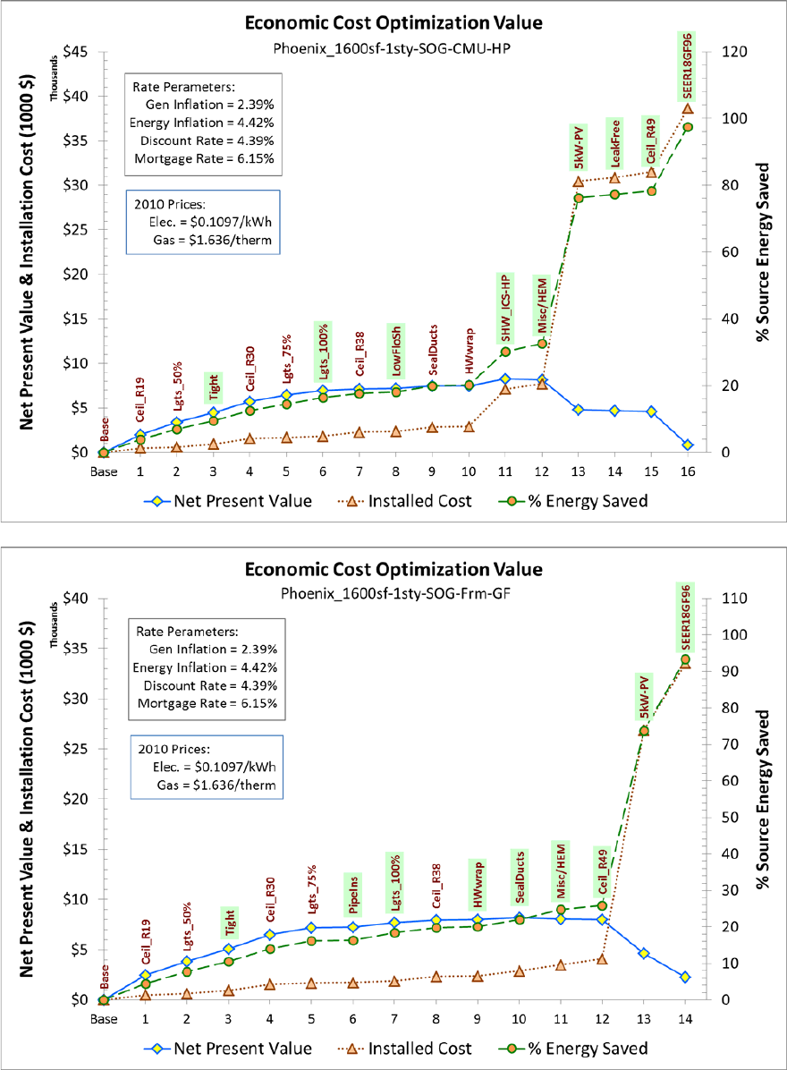
65
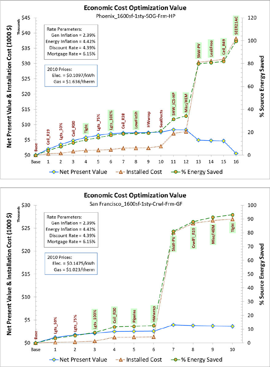
66
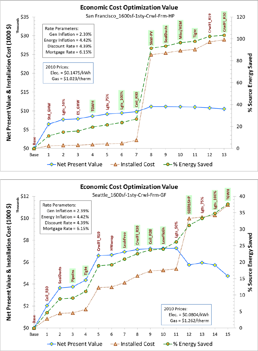
67
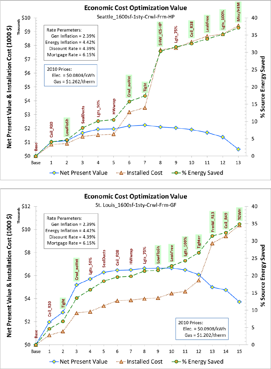
68
69
Appendix D. Optimization Scenario 2—
Homeowner Financing Home Improvement Loan
Model
The figures shown on the following pages are in a standard CostOpt format that plots the
cumulative investment costs and the cumulative NPV of the investments on the left-hand vertical
axis and the cumulative source energy savings percentage on the right-hand axis. Thus, if an
individual improvement measure has an SIR greater than unity, cumulative NPV will increase.
However, if an individual measure has an SIR less than unity, cumulative NPV will decrease.
Therefore, the point at which the NPV is largest is the optimum cost effectiveness from the
consumer’s perspective. However, often measures come in at the end of the optimization that
have an individual measure SIR less than unity but that do not cause the cumulative NPV to drop
below zero. These measures are also cost effective from a societal perspective in that they are
“paid for” by the earlier highly cost-effective measures. Thus, the neutral cost point from the
CostOpt perspective is the line where the cumulative NPV equals zero. Because the optimization
method is incremental, a number of measures are selected and then later replaced by higher
efficiency measures in the same category. Thus, for ease of understanding, the final selections in
each category are highlighted in light green on the plots.
Key to acronyms:
1600sf: Archetype home size in square feet
1sty: One-story above grade home
SOG: Slab-on-grade foundation
Crwl: Crawlspace foundation
Bsmt: Unconditioned basement foundation
HP: Electric space and water heating in base archetype
GF: Natural gas space and water heating in base archetype
7-yr: Seven year mortgage period (used in Scenarios 2 and 3)
incHVAC: Incremental costs used for HVAC systems (used in Scenario 3)
ReFi: Refinance scenario using 4% mortgage interest (used in Scenario 4)
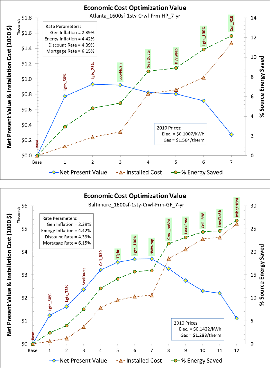
70
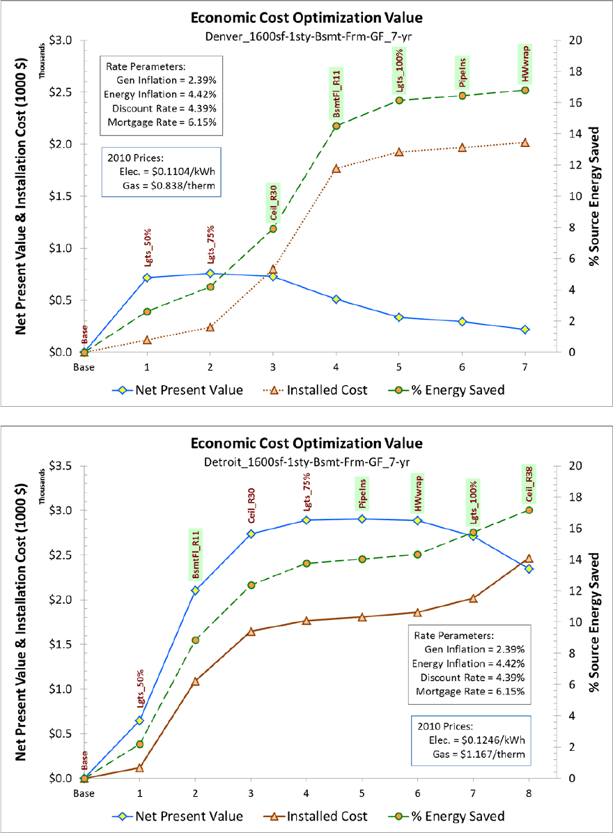
71
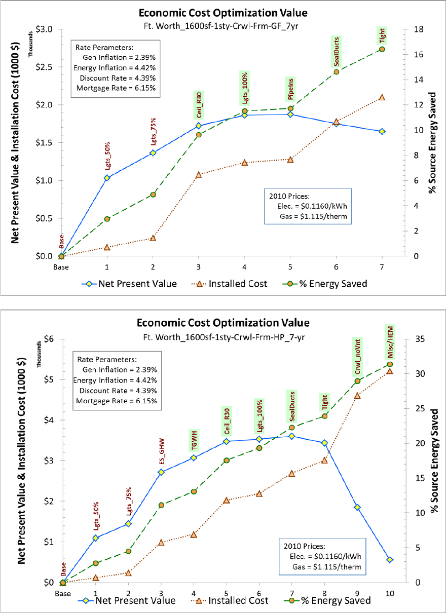
72
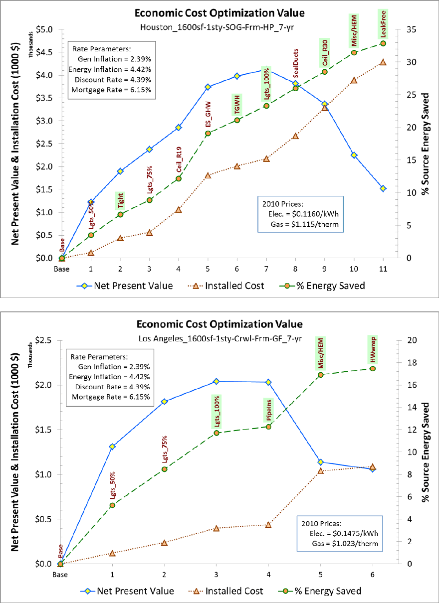
73
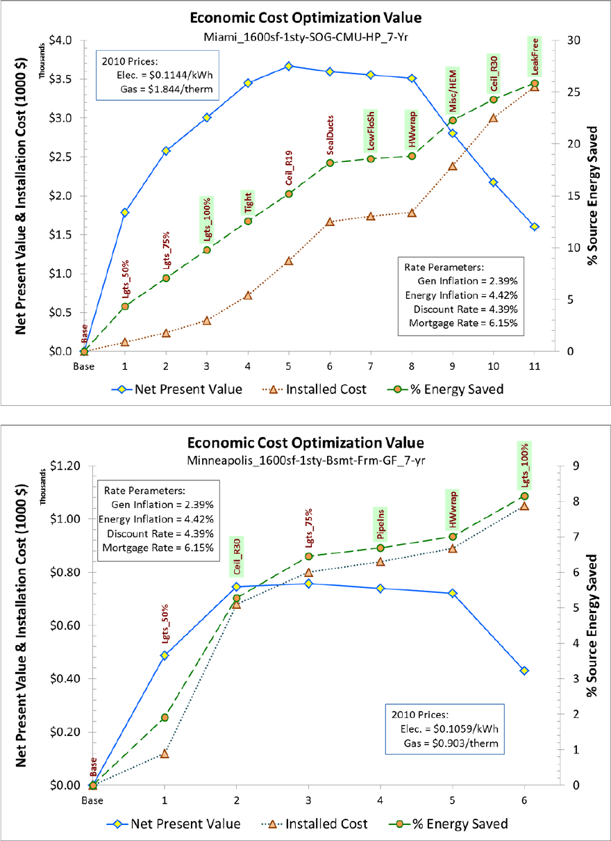
74
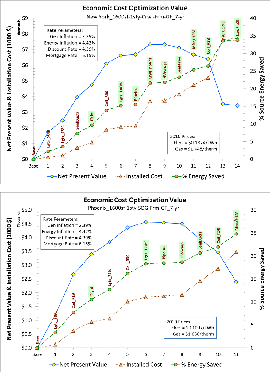
75
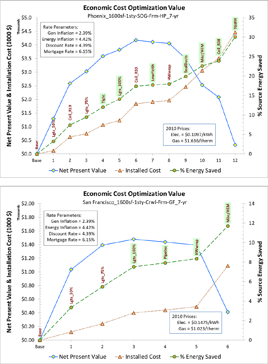
76
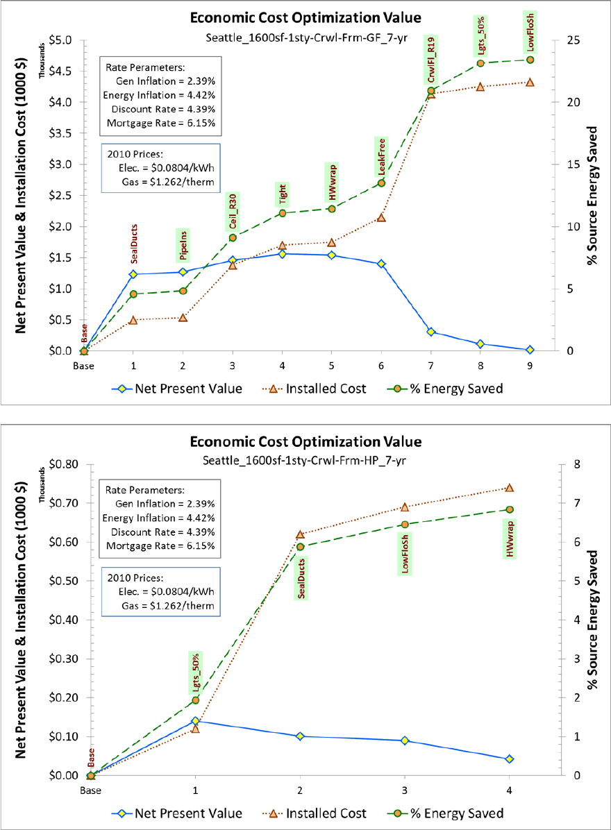
77
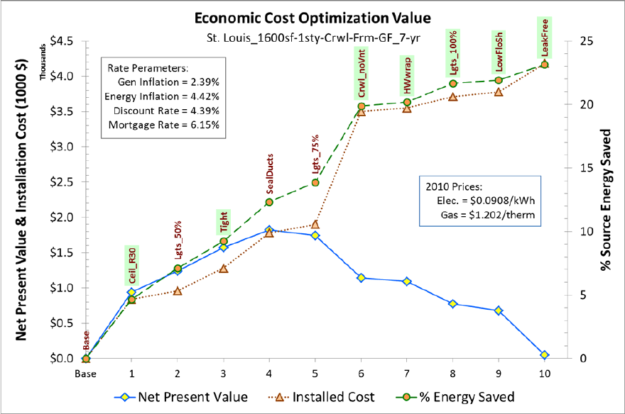
78
79
Appendix E. Optimization Scenario 3—
HVAC Contractor Financing Business Model
The figures shown on the following pages are in a standard CostOpt format that plots the
cumulative investment costs and the cumulative NPV of the investments on the left-hand vertical
axis and the cumulative source energy savings percentage on the right-hand axis. Thus, if an
individual improvement measure has an SIR greater than unity, cumulative NPV will increase.
However, if an individual measure has an SIR less than unity, cumulative NPV will decrease.
Therefore, the point at which the NPV is largest is the optimum cost effectiveness from the
consumer’s perspective. However, often measures come in at the end of the optimization that
have an individual measure SIR less than unity but that do not cause the cumulative NPV to drop
below zero. These measures are also cost effective from a societal perspective in that they are
“paid for” by the earlier highly cost-effective measures. Thus, the neutral cost point from the
CostOpt perspective is the line where the cumulative NPV equals zero. Because the optimization
method is incremental, a number of measures are selected and then later replaced by higher
efficiency measures in the same category. Thus, for ease of understanding, the final selections in
each category are highlighted in light green on the plots.
Key to acronyms:
1600sf: Archetype home size in square feet
1sty: One-story above grade home
SOG: Slab-on-grade foundation
Crwl: Crawlspace foundation
Bsmt: Unconditioned basement foundation
HP: Electric space and water heating in base archetype
GF: Natural gas space and water heating in base archetype
7-yr: Seven year mortgage period (used in Scenarios 2 and 3)
incHVAC: Incremental costs used for HVAC systems (used in Scenario 3)
ReFi: Refinance scenario using 4% mortgage interest (used in Scenario 4)
80
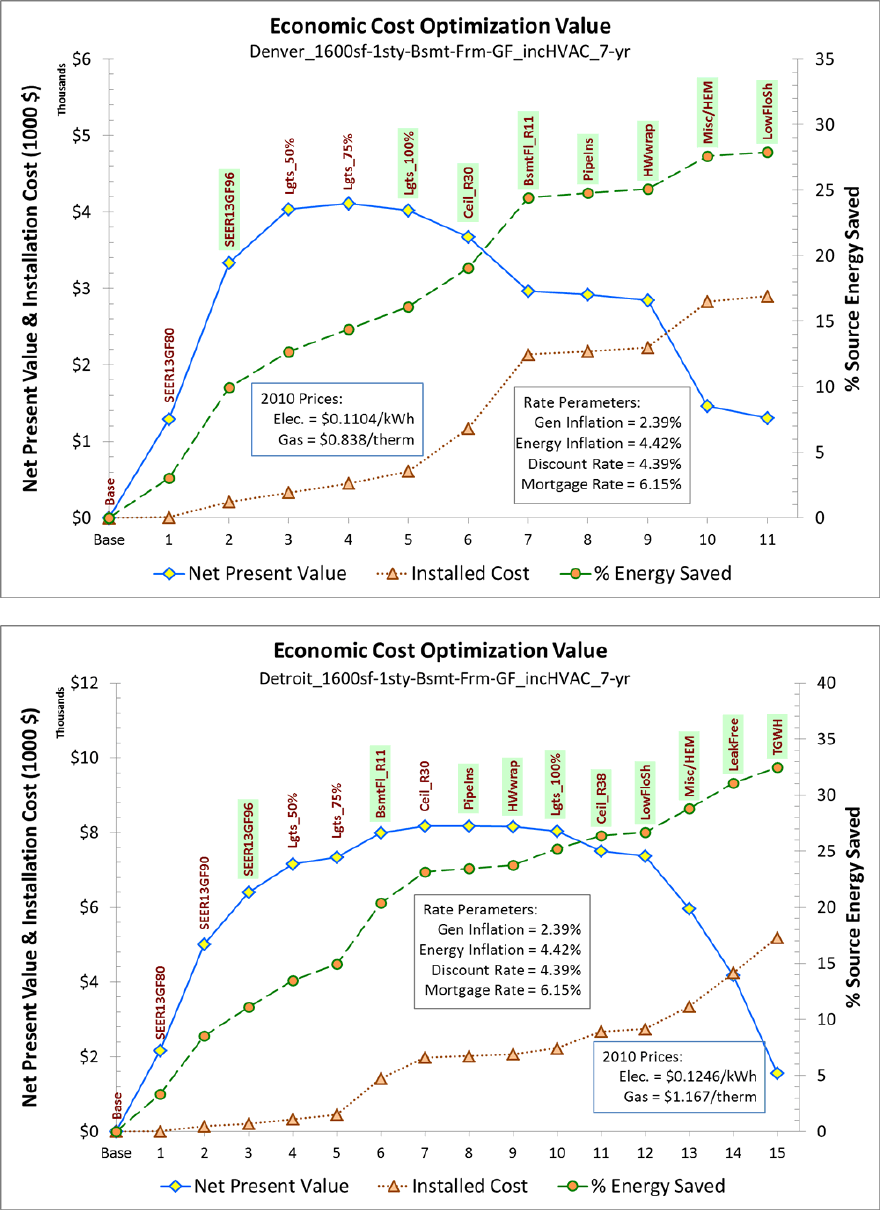
81
82
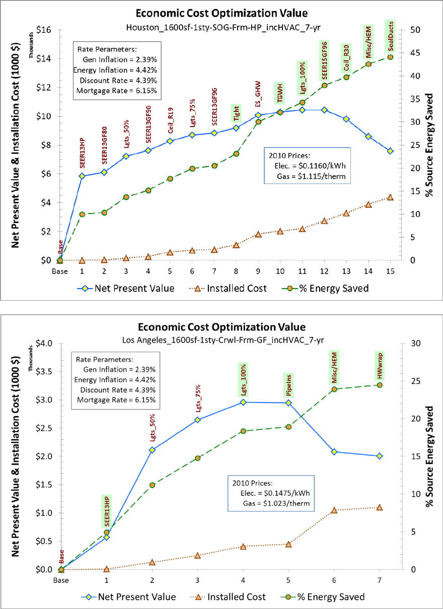
83
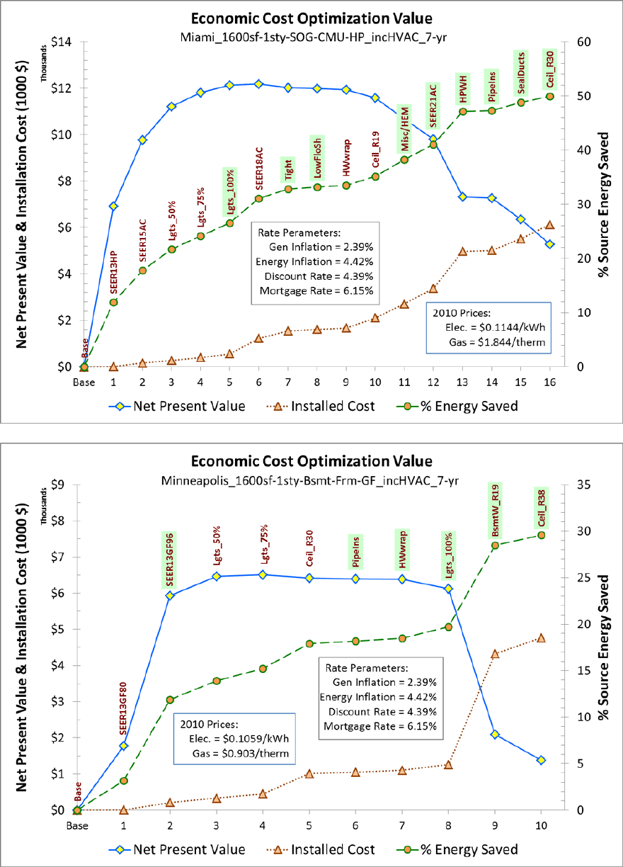
84
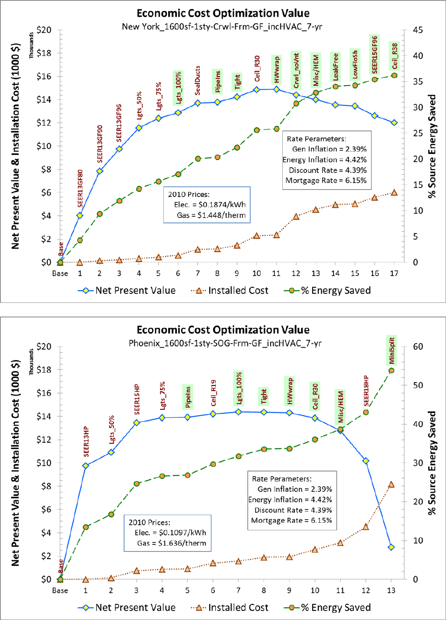
85
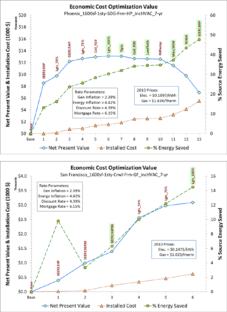
86
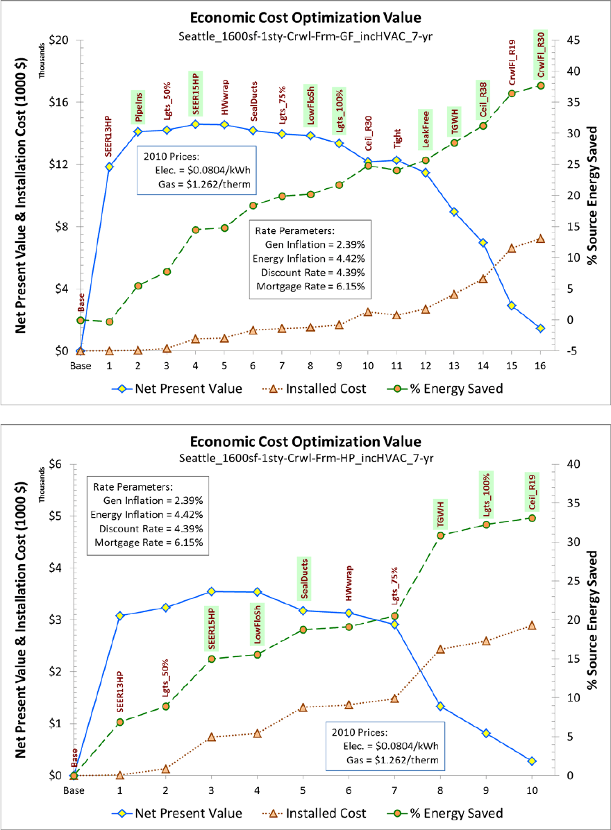
87
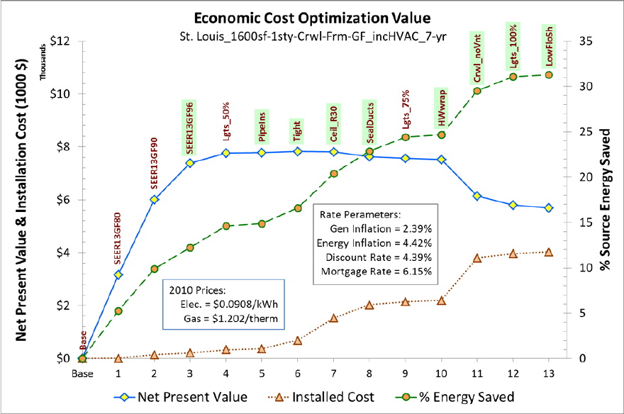
88
89
Appendix F. Optimization Scenario 4—
Home Remodel/Refinance
The figures shown on the following pages are in a standard CostOpt format that plots the
cumulative investment costs and the cumulative Net Present Value (NPV) of the investments on
the left-hand vertical axis and the cumulative source energy savings percentage on the right-hand
axis. Thus, if an individual improvement measure has a Saving-to-Investment Ratio (SIR) greater
than unity, cumulative NPV will increase. However, if an individual measure has an SIR less
than unity, cumulative NPV will decrease. Therefore, the point at which the NPV is largest is the
optimum cost effectiveness from the consumer’s perspective. However, often there are measures
that come in at the end of the optimization which have an individual measure SIR less than unity
but which do not cause the cumulative NPV to drop below zero. These measures are also cost
effective from a societal perspective in that they are “paid for” by the earlier highly cost effective
measures. Thus, the neutral cost point from the CostOpt perspective is the line where the
cumulative NPV equals zero. Since the optimization method is incremental there also are a
number of measures that are selected and then later replaced by measures in the same category
with greater levels of efficiency. Thus, for ease of understanding, the final selections in each
category are highlighted in light green on the plots.
Key to acronyms:
1600sf: Archetype home size in square feet
1sty: One-story above grade home
SOG: Slab-on-grade foundation
Crwl: Crawlspace foundation
Bsmt: Unconditioned basement foundation
HP: Electric space and water heating in base archetype
GF: Natural gas space and water heating in base archetype
7-yr: Seven year mortgage period (used in Scenarios 2 and 3)
incHVAC: Incremental costs used for HVAC systems (used in Scenario 3)
ReFi: Refinance scenario using 4% mortgage interest (used in Scenario 4)
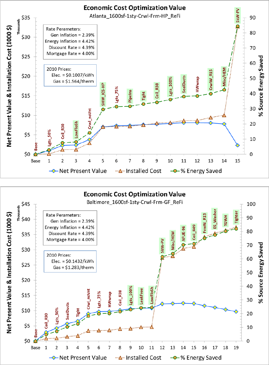
90
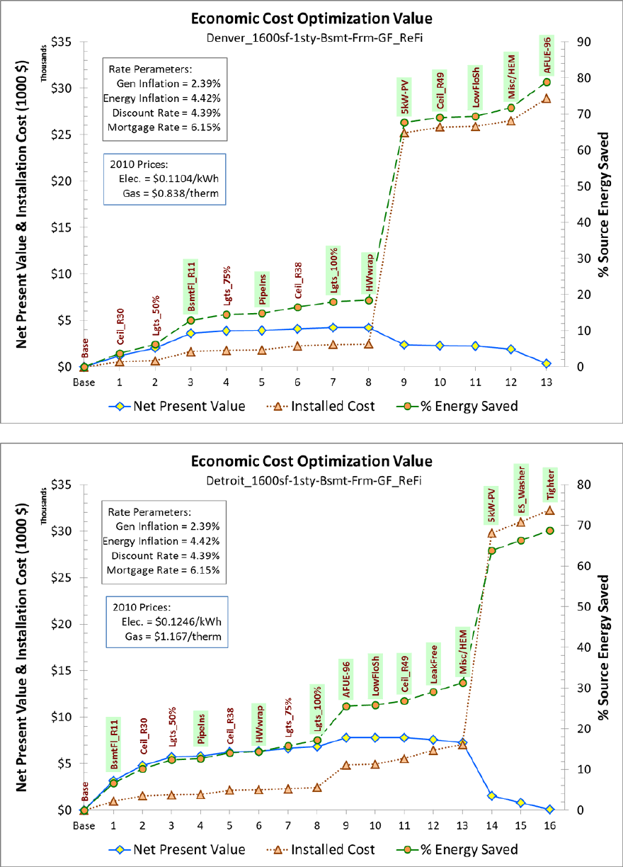
91
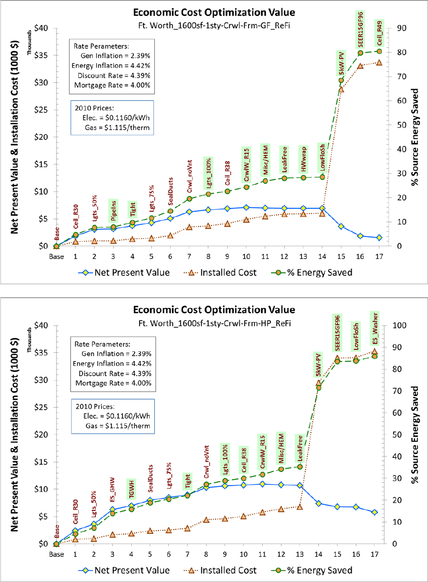
92
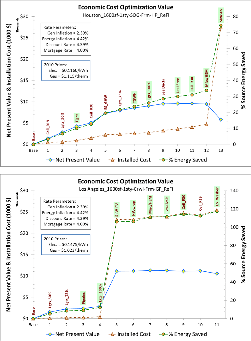
93
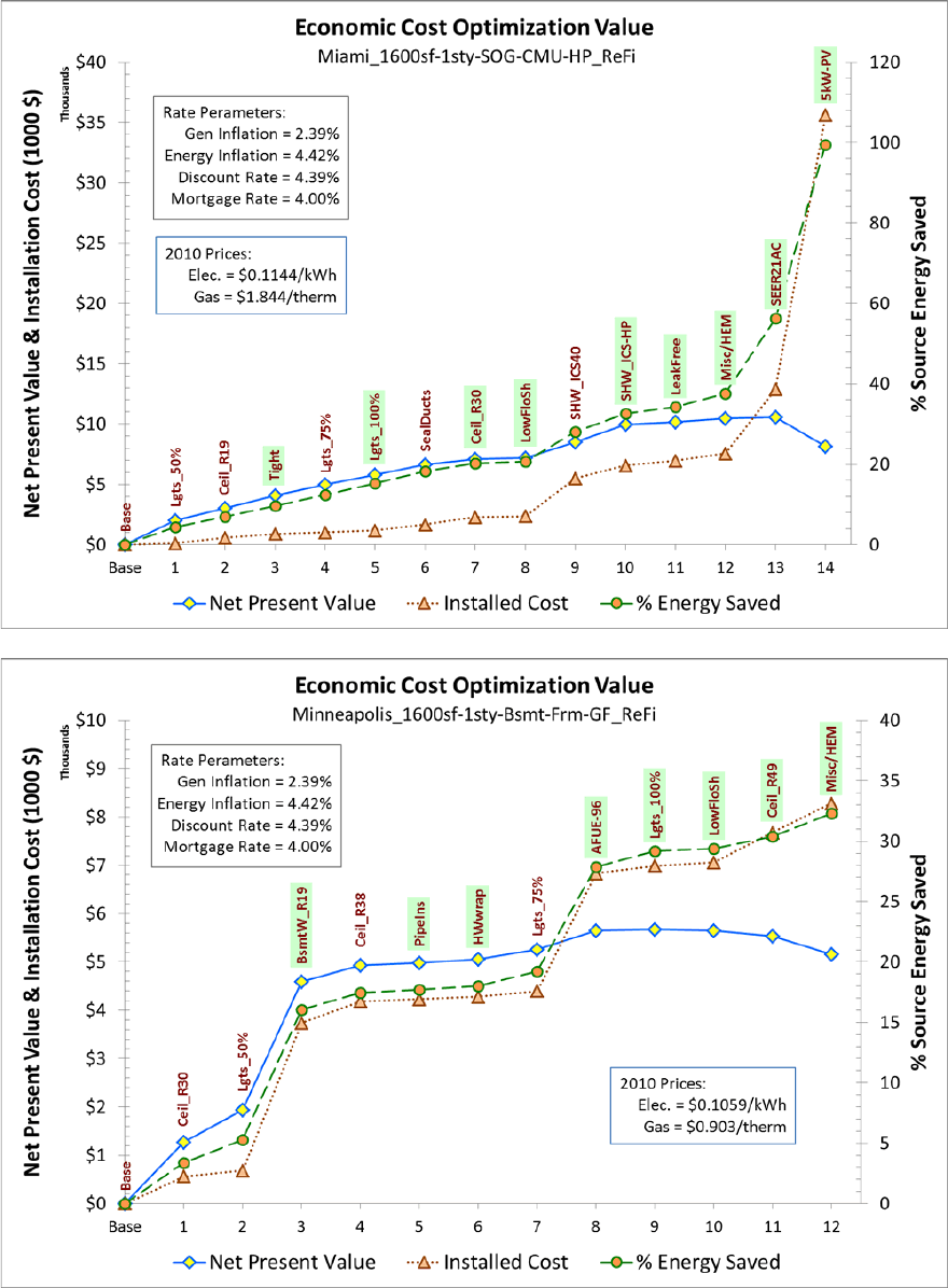
94
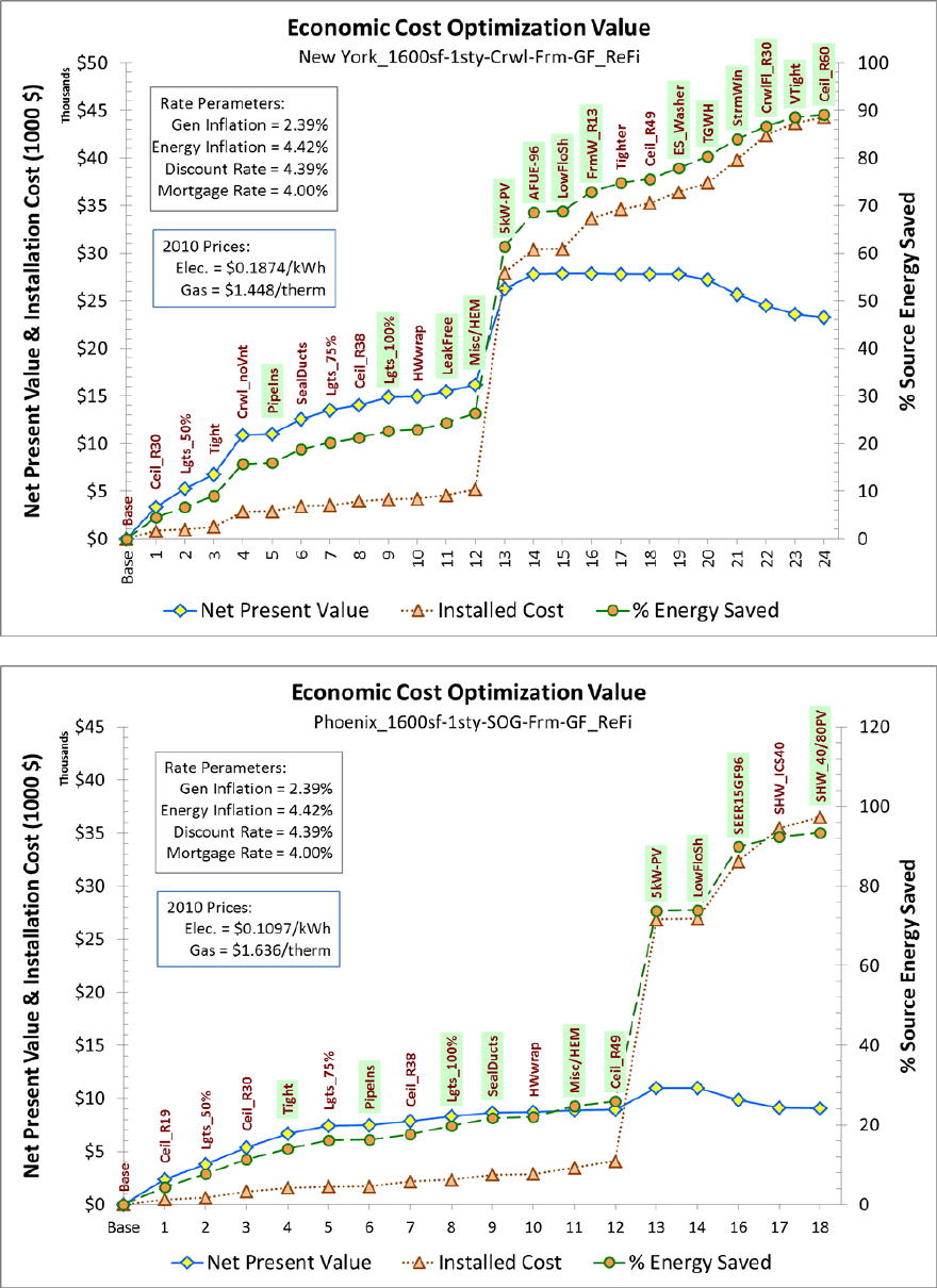
95
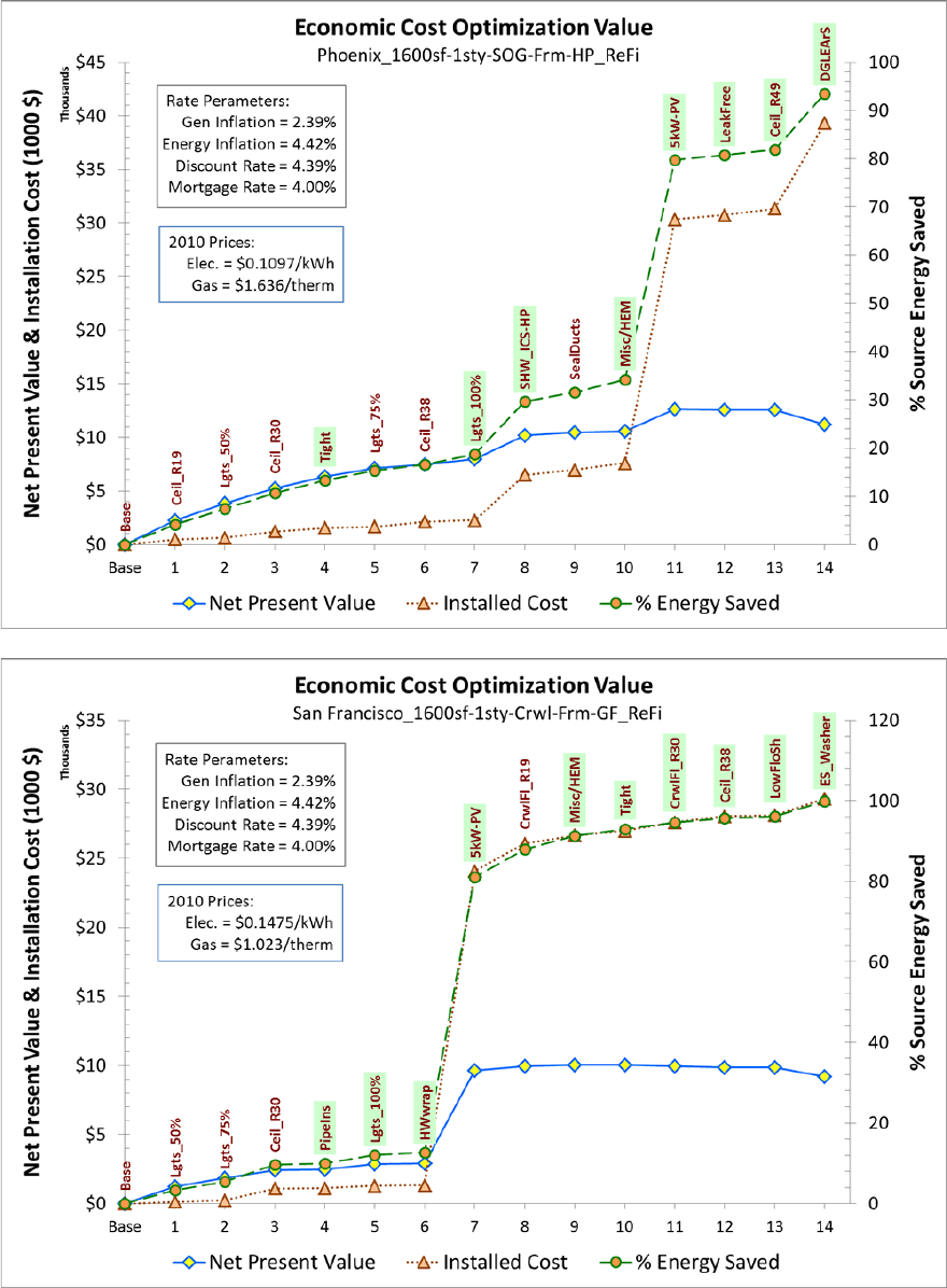
96
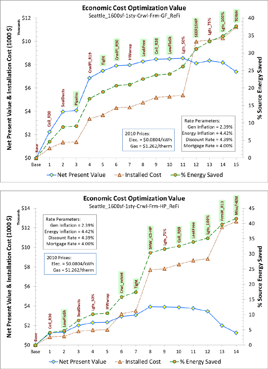
97
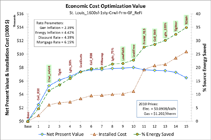
98

DOE/GO-102012-3786 ▪ November 2012
Printed with a renewable-source ink on paper containing at
least 50% wastepaper, including 10% post-consumer waste.
